序言
我们通常用线条来绘制2D图形,大致分为两种线条:直线和曲线。不论我们动手还是用电脑,都能很容易地画出第一种线条。只要给电脑起点和终点,砰!直线就画出来了。没什么好疑问的。
然而,绘制曲线却是个大问题。虽然我们可以很容易地徒手画出曲线,但除非给出描述曲线的数学函数,不然计算机无法画出曲线。实际上,画直线时也需要数学函数,但画直线所需的方程式很简单,我们在这里不去考虑。在计算机看来,所有线条都是“函数”,不管它们是直线还是曲线。然而,这就表示我们需要找到能在计算机上表现良好的曲线方程。这样的曲线有很多种,在本文我们主要关注一类特殊的、备受关注的函数,基本上任何画曲线的地方都会用到它:贝塞尔曲线。
它们是以Pierre Bézier命名的,尽管他并不是第一个,或者说唯一“发明”了这种曲线的人,但他让世界知道了这种曲线十分适合设计工作(在1962年为Renault工作并发表了他的研究)。有人也许会说数学家Paul de Casteljau是第一个发现这类曲线特性的人,在Citroën工作时,他提出了一种很优雅的方法来画这些曲线。然而,de Casteljau没有发表他的工作,这使得“谁先发现”这一问题很难有一个确切的答案。 贝塞尔曲线本质上是伯恩斯坦多项式,这是Sergei Natanovich Bernstein研究的一种数学函数,关于它们的出版物至少可以追溯到1912年。无论如何,这些都只是一些冷知识,你可能更在意的是这些曲线很方便:你可以连接多条贝塞尔曲线,并且连接起来的曲线看起来就像是一条曲线。甚至,在你在Photoshop中画“路径”或使用一些像Flash、Illustrator和Inkscape这样的矢量绘图程序时,所画的曲线都是贝塞尔曲线。
那么,要是你自己想编程实现它们呢?有哪些陷阱?你怎么画它们?包围盒是怎么样的,怎么确定交点,怎么拉伸曲线,简单来说:你怎么对曲线做一切你想做的事?这就是这篇文章想说的。准备好学习一些数学吧!
注意:几乎所有的贝塞尔图形都是可交互的。
这个页面使用了基于Bezier.js 的可交互例子。
这本书是开源的。
这本书是开源的软件项目,现有两个github仓库。第一个https://github.com/pomax/bezierinfo,它是你现在在看的这个,纯粹用来展示的版本。另外一个https://github.com/pomax/BezierInfo-2,是带有所有html, javascript和css的开发版本。你可以fork任意一个,随便做些什么,当然除了把它当作自己的作品来商用。 =)
用到的数学将有多复杂?
这份入门读物用到的大部分数学知识都是高中所学的。如果你理解基本的计算并能看懂英文的话,就能上手这份材料。有时候会用到复杂一点的数学,但如果你不想深究它们,可以选择跳过段落里的“详解”部分,或者直接跳到章节末尾,避开那些看起来很深入的数学。章节的末尾往往会列出一些结论,因此你可以直接利用这些结论。
问题,评论:
如果你有对于新章节的一些建议,点击 Github issue tracker (也可以点右上角的repo链接)。如果你有关于材料的一些问题,由于我现在在做改写工作,目前没有评论功能,但你可以用issue跟踪来发表评论。一旦完成重写工作,我会把评论功能加上,或者会有“选择文字段落,点击‘问题’按钮来提问”的系统。到时候我们看看。
给我买杯咖啡?
如果你很喜欢这本书,或发现它对你要做的事很有帮助,或者你想知道怎么表达自己对这本书的感激,你可以 给我买杯咖啡 ,所少钱取决于你。这份工作持续了很多年,从一份小小的简要到70多页关于贝塞尔曲线的读物,在完成它的过程中倾注了很多咖啡。我从未后悔花在这上面的每一分钟,但如果有更多咖啡的话,我可以坚持写下去!
变更日志
本入门是一份活动文档,因此它可能会有新的内容,这取决于你上次查看的时间。单击以下链接以展开,查看添加的内容、时间,或点击浏览 News posts 获取更多更新信息。 (RSS feed 可用)
November 2020
Added a section on finding curve/circle intersections
October 2020
Added the Ukranian locale! Help out in getting its localization to 100%!
August-September 2020
-
Completely overhauled the site: the Primer is now a normal web page that works fine with JS disabled, but obviously better with JS turned on.
June 2020
Added automatic CI/CD using Github Actions
January 2020
Added reset buttons to all graphics
Updated to preface to correctly describe the on-page maths
Fixed the Catmull-Rom section because it had glaring maths errors
August 2019
Added a section on (plain) rational Bezier curves
Improved the Graphic component to allow for sliders
December 2018
Added a section on curvature and calculating kappa.
-
Added a Patreon page! Head on over to patreon.com/bezierinfo to help support this site!
August 2018
Added a section on finding a curve's y, if all you have is the x coordinate.
July 2018
Rewrote the 3D normals section, implementing and explaining Rotation Minimising Frames.
Updated the section on curve order raising/lowering, showing how to get a least-squares optimized lower order curve.
-
(Finally) updated 'npm test' so that it automatically rebuilds when files are changed while the dev server is running.
June 2018
Added a section on direct curve fitting.
Added source links for all graphics.
Added this "What's new?" section.
April 2017
Added a section on 3d normals.
Added live-updating for the social link buttons, so they always link to the specific section you're reading.
February 2017
Finished rewriting the entire codebase for localization.
January 2016
Added a section to explain the Bezier interval.
Rewrote the Primer as a React application.
December 2015
Set up the split repository between BezierInfo-2 as development repository, and bezierinfo as live page.
-
Removed the need for client-side LaTeX parsing entirely, so the site doesn't take a full minute or more to load all the graphics.
May 2015
Switched over to pure JS rather than Processing-through-Processing.js
Added Cardano's algorithm for finding the roots of a cubic polynomial.
April 2015
Added a section on arc length approximations.
February 2015
Added a section on the canonical cubic Bezier form.
November 2014
Switched to HTTPS.
July 2014
Added the section on arc approximation.
April 2014
Added the section on Catmull-Rom fitting.
November 2013
Added the section on Catmull-Rom / Bezier conversion.
Added the section on Bezier cuves as matrices.
April 2013
Added a section on poly-Beziers.
Added a section on boolean shape operations.
March 2013
First drastic rewrite.
Added sections on circle approximations.
Added a section on projecting a point onto a curve.
Added a section on tangents and normals.
Added Legendre-Gauss numerical data tables.
October 2011
-
First commit for the bezierinfo site, based on the pre-Primer webpage that covered the basics of Bezier curves in HTML with Processing.js examples.
简单介绍
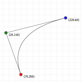
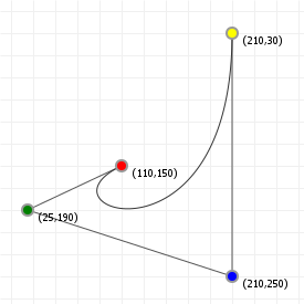
让我们有个好的开始:当我们在谈论贝塞尔曲线的时候,所指的就是你在如下图像看到的东西。它们从某些起点开始,到终点结束,并且受到一个或多个的“中间”控制点的影响。本页面上的图形都是可交互的,你可以拖动这些点,看看这些形状在你的操作下会怎么变化。
这些曲线在计算机辅助设计和计算机辅助制造应用(CAD/CAM)中用的很多。在图形设计软件中也常用到,像Adobe Illustrator, Photoshop, Inkscape, Gimp等等。还可以应用在一些图形技术中,像矢量图形(SVG)和OpenType字体(ttf/otf)。许多东西都用到贝塞尔曲线,如果你想更了解它们...准备好继续往下学吧!
什么构成了贝塞尔曲线?
操作点的移动,看看曲线的变化,可能让你感受到了贝塞尔曲线是如何表现的。但贝塞尔曲线究竟是什么呢?有两种方式来解释贝塞尔曲线,并且可以证明它们完全相等,但是其中一种用到了复杂的数学,另外一种比较简单。所以...我们先从简单的开始吧:
贝塞尔曲线是线性插值的结果。这听起来很复杂,但你在很小的时候就做过线性插值:当你指向两个物体中的另外一个物体时,你就用到了线性插值。它就是很简单的“选出两点之间的一个点”。
如果我们知道两点之间的距离,并想找出离第一个点20%间距的一个新的点(也就是离第二个点80%的间距),我们可以通过简单的计算来得到:

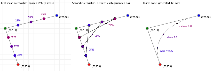
让我们来通过实际操作看一下:下面的图形都是可交互的,因此你可以通过上下键来增加或减少插值距离,来观察图形的变化。我们从三个点构成的两条线段开始。通过对各条线段进行线性插值得到两个点,对点之间的线段再进行线性插值,产生一个新的点。最终这些点——所有的点都可以通过选取不同的距离插值产生——构成了贝塞尔曲线:
这为我们引出了复杂的数学:微积分。
虽然我们刚才好像没有用到这个,我们实际上只是逐步地画了一条二次曲线,而不是一次画好。贝塞尔曲线的一个很棒的特性就是它们可以通过多项式方程表示,也可以用很简单的插值形式表示。因此,反过来说,我们可以基于“真正的数学”(检查方程式,导数之类的东西),也可以通过观察曲线的“机械”构成(比如说,可以得知曲线永远不会延伸超过我们用来构造它的点),来看看这些曲线能够做什么。
让我们从更深的层次来观察贝塞尔曲线。看看它们的数学表达式,从这些表达式衍生得到的属性,以及我们可以对贝塞尔曲线做的事。
贝塞尔曲线的数学原理
贝塞尔曲线是“参数”方程的一种形式。从数学上讲,参数方程作弊了:“方程”实际上是一个从输入到唯一输出的、良好定义的映射关系。几个输入进来,一个输出返回。改变输入变量,还是只有一个输出值。参数方程在这里作弊了。它们基本上干了这么件事,“好吧,我们想要更多的输出值,所以我们用了多个方程”。举个例子:假如我们有一个方程,通过一些计算,将假设为x的一些值映射到另外的值:

记号f(x)是表示函数的标准方式(为了方便起见,如果只有一个的话,我们称函数为f),函数的输出根据一个变量(本例中是x)变化。改变x,f(x)的输出值也会变。
到目前没什么问题。现在,让我们来看一下参数方程,以及它们是怎么作弊的。我们取以下两个方程:

这俩方程没什么让人印象深刻的,只不过是正弦函数和余弦函数,但正如你所见,输入变量有两个不同的名字。如果我们改变了a的值,f(b)的输出不会有变化,因为这个方程没有用到a。参数方程通过改变这点来作弊。在参数方程中,所有不同的方程共用一个变量,如下所示:

多个方程,但只有一个变量。如果我们改变了t的值,fa(t)和fb(t)的输出都会发生变化。你可能会好奇这有什么用,答案其实很简单:对于参数曲线,如果我们用常用的标记来替代fa(t)和fb(t),看起来就有些明朗了:

好了,通过一些神秘的t值将x/y坐标系联系起来。
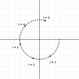
所以,参数曲线不像一般函数那样,通过x坐标来定义y坐标,而是用一个“控制”变量将它们连接起来。如果改变t的值,每次变化时我们都能得到两个值,这可以作为图形中的(x,y)坐标。比如上面的方程组,生成位于一个圆上的点:我们可以使t在正负极值间变化,得到的输出(x,y)都会位于一个以原点(0,0)为中心且半径为1的圆上。如果我们画出t从0到5时的值,将得到如下图像:
贝塞尔曲线是(一种)参数方程,并在它的多个维度上使用相同的基本方程。在上述的例子中x值和y值使用了不同的方程,与此不同的是,贝塞尔曲线的x和y都用了“二项多项式”。那什么是二项多项式呢?
你可能记得高中所学的多项式,看起来像这样:

如果它的最高次项是x³就称为“三次”多项式,如果最高次项是x²,称为“二次”多项式,如果只含有x的项,它就是一条线(不过不含任何x的项它就不是一个多项式!)
贝塞尔曲线不是x的多项式,它是t的多项式,t的值被限制在0和1之间,并且含有a,b等参数。它采用了二次项的形式,听起来很神奇但实际上就是混合不同值的简单描述:

我明白你在想什么:这看起来并不简单,但如果我们拿掉t并让系数乘以1,事情就会立马简单很多,看看这些二次项:

需要注意的是,2与1+1相同,3相当于2+1或1+2,6相当于3+3...如你所见,每次我们增加一个维度,只要简单地将头尾置为1,中间的操作都是“将上面的两个数字相加”。现在就能很容易地记住了。
还有一个简单的办法可以弄清参数项怎么工作的:如果我们将(1-t)重命名为a,将t重命名为b,暂时把权重删掉,可以得到这个:

基本上它就是“每个a和b结合项”的和,在每个加号后面逐步的将a换成b。因此这也很简单。现在你已经知道了二次多项式,为了叙述的完整性,我将给出一般方程:

这就是贝塞尔曲线完整的描述。在这个函数中的Σ表示了这是一系列的加法(用Σ下面的变量,从...=<值>开始,直到Σ上面的数字结束)。
如何实现基本方程
我们可以用之前说过的方程,来简单地实现基本方程作为数学构造,如下:
| 1 | |
| 2 | |
| 3 | |
| 4 | |
| 5 |
我说我们“可以用”是因为我们不会这么去做:因为阶乘函数开销非常大。并且,正如我们在上面所看到的,我们不用阶乘也能够很容易地构造出帕斯卡三角形:一开始是[1],接着是[1,2,1],然后是[1,3,3,1]等等。下一行都比上一行多一个数,首尾都为1,中间的数字是上一行两边元素的和。
我们可以很快的生成这个列表,并在之后使用这个查找表而不用再计算二次多项式的系数:
| 1 | |
| 2 | |
| 3 | |
| 4 | |
| 5 | |
| 6 | |
| 7 | |
| 8 | |
| 9 | |
| 10 | |
| 11 | |
| 12 | |
| 13 | |
| 14 | |
| 15 | |
| 16 | |
| 17 | |
| 18 |
这里做了些什么?首先,我们声明了一个足够大的查找表。然后,我们声明了一个函数来获取我们想要的值,并且确保当一个请求的n/k对不在LUT查找表中时,先将表扩大。我们的基本函数如下所示:
| 1 | |
| 2 | |
| 3 | |
| 4 | |
| 5 |
完美。当然我们可以进一步优化。为了大部分的计算机图形学目的,我们不需要任意的曲线。我们需要二次曲线和三次曲线(实际上这篇文章没有涉及任意次的曲线,因此你会在其他地方看到与这些类似的代码),这说明我们可以彻底简化代码:
| 1 | |
| 2 | |
| 3 | |
| 4 | |
| 5 | |
| 6 | |
| 7 | |
| 8 | |
| 9 | |
| 10 | |
| 11 | |
| 12 | |
| 13 |
现在我们知道如何代用码实现基本方程了。很好。
既然我们已经知道基本函数的样子,是时候添加一些魔法来使贝塞尔曲线变得特殊了:控制点。
控制贝塞尔的曲率
贝塞尔曲线是插值方程(就像所有曲线一样),这表示它们取一系列的点,生成一些处于这些点之间的值。(一个推论就是你永远无法生成一个位于这些控制点轮廓线外面的点,更普遍是称为曲线的外壳。这信息很有用!)实际上,我们可以将每个点对方程产生的曲线做出的贡献进行可视化,因此可以看出曲线上哪些点是重要的,它们处于什么位置。
下面的图形显示了二次曲线和三次曲线的差值方程,“S”代表了点对贝塞尔方程总和的贡献。点击拖动点来看看在特定的t值时,每个曲线定义的点的插值百分比。
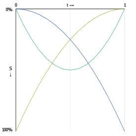
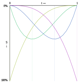
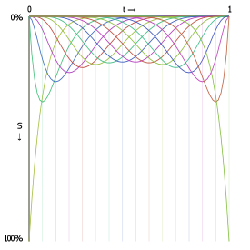
上面有一张是15th阶的插值方程。如你所见,在所有控制点中,起点和终点对曲线形状的贡献比其他点更大些。
如果我们要改变曲线,就需要改变每个点的权重,有效地改变插值。可以很直接地做到这个:只要用一个值乘以每个点,来改变它的强度。这个值照惯例称为“权重”,我们可以将它加入我们原始的贝塞尔函数:

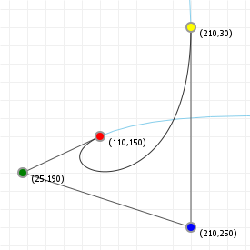
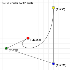
看起来很复杂,但实际上“权重”只是我们想让曲线所拥有的坐标值:对于一条nth阶曲线,w0是起始坐标,wn是终点坐标,中间的所有点都是控制点坐标。假设说一条曲线的起点为(110,150),终点为(210,30),并受点(25,190)和点(210,250)的控制,贝塞尔曲线方程就为:

这就是我们在文章开头看到的曲线:
我们还能对贝塞尔曲线做些什么?实际上还有很多。文章接下来涉及到我们可能运用到的一系列操作和算法,以及它们可以完成的任务。
如何实现权重基本函数
鉴于我们已经知道怎样实现基本函数,在其加入控制点是非常简单的:
| 1 | |
| 2 | |
| 3 | |
| 4 | |
| 5 |
下面是优化过的版本:
| 1 | |
| 2 | |
| 3 | |
| 4 | |
| 5 | |
| 6 | |
| 7 | |
| 8 | |
| 9 | |
| 10 | |
| 11 | |
| 12 | |
| 13 |
现在我们知道如何编程实现基本权重函数了。
控制贝塞尔曲线的曲率,第二部分:有理贝塞尔
我们可以通过“有理化”来进一步控制贝塞尔曲线,即,除了在上一小节中讨论的权重外,还通过添加“比率”参数来调节每个控制点对曲线影响的“强度”。
常规的贝塞尔曲线函数表达式如下:

将比率添加到其中非常容易,只需要添加两项。有理贝塞尔曲线函数表达式如下:

这里,第一个新添项表示的是每个控制点的一个“额外的”权重。例如,如果比率为[1,0.5,0.5,1],那么ratio0 = 1,
ratio1 = 0.5,以此类推。可见,这就好比使用了“双重加权”,并没有什么特别之处。
特别之处在于第二个新添项:曲线上的每个点不仅仅是一个“双重加权”点,它是通过引入比率计算的“双重加权”值的一个分数。当计算曲线上的点时,我们先计算“常规的”贝塞尔值,然后除以用比率,而不是权重计算出来的新曲线的贝塞尔值。
这会产生一些意想不到的结果:它把多项式变成了非多项式的表达式。它现在是一种由多项式的超类表示的曲线,能够实现一些贝塞尔曲线本身无法实现的很酷的事情,例如准确地描述圆形(稍后会看到,这是贝塞尔曲线无法做到的。)
展示贝塞尔曲线有理化作用的最佳方法还是使用交互式图片来查看效果。下方图片显示的是前序小节中使用的贝塞尔曲线的每个控制点添加了比率的结果。比率值越接近于0,相关控制点对曲线的相对影响就越小,反之亦然。请尝试更改这些比率值并观察它们如何影响曲线:

你可以把比率想象为每个控制点的“重力”:重力越大,曲线就越接近该控制点。你还会注意到,如果只是将所有比率都增加或减少相同的值,则曲线不会发生任何变化。就像重力一样,如果相对强度保持不变,则不会发生任何真正的变化。这些值决定了每个控制点对其他点的影响。
如何实现有理化曲线
给前序小节的代码添加比率只需要一些小改动:
| 1 | |
| 2 | |
| 3 | |
| 4 | |
| 5 | |
| 6 | |
| 7 | |
| 8 | |
| 9 | |
| 10 | |
| 11 | |
| 12 | |
| 13 | |
| 14 | |
| 15 | |
| 16 | |
| 17 | |
| 18 | |
| 19 | |
| 20 | |
| 21 | |
| 22 | |
| 23 | |
| 24 | |
| 25 | |
| 26 |
这就是我们需要做的全部。
贝塞尔区间[0,1]
既然我们知道了贝塞尔曲线背后的数学原理,你可能会注意到一件奇怪的事:它们都是从t=0到t=1。为什么是这个特殊区间?
这一切都与我们如何从曲线的“起点”变化到曲线“终点”有关。如果有一个值是另外两个值的混合,一般方程如下:

很显然,起始值需要a=1, b=0,混合值就为100%的value 1和0%的value 2。终点值需要a=0, b=1,则混合值是0%的value
1和100%的value
2。另外,我们不想让“a”和“b”是互相独立的:如果它们是互相独立的话,我们可以任意选出自己喜欢的值,并得到混合值,比如说100%的value1和100%的value2。原则上这是可以的,但是对于贝塞尔曲线来说,我们通常想要的是起始值和终点值之间的混合值,所以要确保我们不会设置一些“a”和"b"而导致混合值超过100%。这很简单:

用这个式子我们可以保证相加的值永远不会超过100%。通过将a限制在区间[0,1],我们将会一直处于这两个值之间(包括这两个端点),并且相加为100%。
但是...如果我们没有假定只使用0到1之间的数,而是用一些区间外的值呢,事情会变得很糟糕吗?好吧...不全是,我们接下来看看。
对于贝塞尔曲线的例子,扩展区间只会使我们的曲线“保持延伸”。贝塞尔曲线是多项式曲线上简单的片段,如果我们选一个更大的区间,会看到曲线更多部分。它们看起来是什么样的呢?
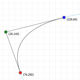
下面两个图形给你展示了以“普通方式”来渲染的贝塞尔曲线,以及如果我们扩大t值时它们所“位于”的曲线。如你所见,曲线的剩余部分隐藏了很多“形状”,我们可以通过移动曲线的点来建模这部分。
实际上,图形设计和计算机建模中还用了一些和贝塞尔曲线相反的曲线,这些曲线没有固定区间和自由的坐标,相反,它们固定座标但给你自由的区间。"Spiro"曲线就是一个很好的例子,它的构造是基于羊角螺线,也就是欧拉螺线的一部分。这是在美学上很令人满意的曲线,你可以在一些图形包中看到它,比如FontForge和Inkscape,它也被用在一些字体设计中(比如Inconsolata字体)。
用矩阵运算来表示贝塞尔曲率
通过将贝塞尔公式表示成一个多项式基本方程、系数矩阵以及实际的坐标,我们也可以用矩阵运算来表示贝塞尔。让我们看一下这对三次曲线来说有什么含义:

暂时不用管我们具体的坐标,现在有:

可以将它写成四个表达式之和:

我们可以扩展这些表达式:

更进一步,我们可以加上所有的1和0系数,以便看得更清楚:

现在,我们可以将它看作四个矩阵运算:

如果我们将它压缩到一个矩阵操作里,就能得到:

这种多项式表达式一般是以递增的顺序来写的,所以我们应该将t矩阵水平翻转,并将大的那个“混合”矩阵上下颠倒:

最终,我们可以加入原始的坐标,作为第三个单独矩阵:

我们可以对二次曲线运用相同的技巧,可以得到:

如果我们代入t值并乘以矩阵来计算,得到的值与解原始多项式方程或用逐步线性插值计算的结果一样。
因此:为什么我们要用矩阵来计算? 用矩阵形式来表达曲线可以让我们去探索函数的一些很难被发现的性质。可以证明的是曲线构成了三角矩阵,并且它与我们用在曲线中的实际坐标的求积相同。它还是可颠倒的,这说明可以满足大量特性。当然,主要问题是:“现在,为什么这些对我们很有用?”,答案就是这些并不是立刻就很有用,但是以后你会看到在一些例子中,曲线的一些属性可以用函数式来计算,也可以巧妙地用矩阵运算来得到,有时候矩阵方法要快得多。
所以,现在只要记着我们可以用这种形式来表示曲线,让我们接着往下看看。
de Casteljau's 算法
要绘制贝塞尔曲线,我们可以从0到1遍历t的所有值,计算权重函数,得到需要画的x/y值。但曲线越复杂,计算量也变得越大。我们可以利用“de
Casteljau算法",这是一种几何画法,并且易于实现。实际上,你可以轻易地用笔和尺画出曲线。
我们用以下步骤来替代用t计算x/y的微积分算法:
- 把
t看做一个比例(实际上它就是),t=0代表线段的0%,t=1代表线段的100%。 - 画出所有点的连线,对
n阶曲线来说可以画出n条线。 - 在每条线的
t处做一个记号。比如t是0.2,就在离起点20%(离终点80%)的地方做个记号。 - 连接
这些点,得到n-1条线。 - 在这些新得到的线上同样用
t为比例标记。 - 把相邻的
那些点连线,得到n-2条线。 - 取记号,连线,取记号,等等。
- 重复这些步骤,直到剩下一条线。这条线段上的
t点就是原始曲线在t处的点。
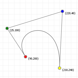
我们通过实际操作来观察这个过程。在以下的图表中,移动鼠标来改变用de Casteljau算法计算得到的曲线点,左右移动鼠标,可以实时看到曲线是如何生成的。
如何实现de Casteljau算法
让我们使用刚才描述过的算法,并实现它:
| 1 | |
| 2 | |
| 3 | |
| 4 | |
| 5 | |
| 6 | |
| 7 | |
| 8 |
好了,这就是算法的实现。一般来说你不能随意重载“+”操作符,因此我们给出计算x和y坐标的实现:
| 1 | |
| 2 | |
| 3 | |
| 4 | |
| 5 | |
| 6 | |
| 7 | |
| 8 | |
| 9 | |
| 10 |
以上算法做了什么?如果参数points列表只有一个点, 就画出一个点。如果有多个点,就生成以t为比例的一系列点(例如,以上算法中的"标记点"),然后为新的点列表调用绘制函数。
简化绘图
我们可以简化绘制的过程,先在具体的位置“采样”曲线,然后用线段把这些点连接起来。由于我们是将曲线转换成一系列“平整的”直线,故将这个过程称之为“拉平(flattening)”。
我们可以先确定“想要X个分段”,然后在间隔的地方采样曲线,得到一定数量的分段。这种方法的优点是速度很快:比起遍历100甚至1000个曲线坐标,我们可以采样比较少的点,仍然得到看起来足够好的曲线。这么做的缺点是,我们失去了“真正的曲线”的精度,因此不能用此方法来做真实的相交检测或曲率对齐。
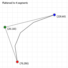
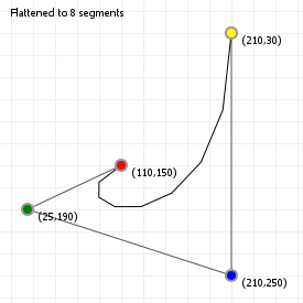
试着点击图形,并用上下键来降低二次曲线和三次曲线的分段数量。你会发现对某些曲率来说,数量少的分段也能做的很好,但对于复杂的曲率(在三次曲线上试试),足够多的分段才能很好地满足曲率的变化。
如何实现曲线的拉平
让我们来实现刚才简述过的算法:
| 1 | |
| 2 | |
| 3 | |
| 4 | |
| 5 | |
| 6 | |
| 7 |
好了,这就是算法的实现。它基本上是画出一系列的线段来模拟“曲线”。
| 1 | |
| 2 | |
| 3 | |
| 4 | |
| 5 | |
| 6 | |
| 7 |
我们将第一个坐标作为参考点,然后在相邻两个点之间画线。
分割曲线
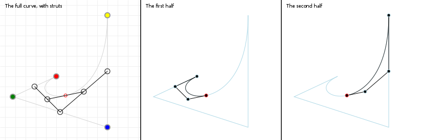
使用 de Casteljau 算法我们也可以将一条贝塞尔曲线分割成两条更小的曲线,二者拼接起来即可形成原来的曲线。当采用某个 t 值构造 de
Casteljau 算法时,该过程会给到我们在 t 点分割曲线的所有点:
一条曲线包含该曲线上点之前的所有点,另一条曲线包含该曲线上点之后的所有点。
分割曲线的代码实习
通过在 de Casteljau 函数里插入一些额外的输出代码,我们就可以实现曲线的分割:
| 1 | |
| 2 | |
| 3 | |
| 4 | |
| 5 | |
| 6 | |
| 7 | |
| 8 | |
| 9 | |
| 10 | |
| 11 | |
| 12 | |
| 13 | |
| 14 | |
| 15 | |
| 16 |
对某个给定 t 值,该函数执行后,数组 left 和 right 将包含两条曲线的所有点的坐标 --
一条是t值左侧的曲线,一条是t值右侧的曲线, 与原始曲线同序且完全重合。
用矩阵分割曲线
另一种分割曲线的方法是利用贝塞尔曲线的矩阵表示。矩阵一章已经说明可以用矩阵乘法表示曲线,尤其是以下两种分别表示二次曲线和三次曲线的形式(为提高可读性,贝塞尔曲线的系数向量已被倒转次序):

和

假设要在点t = z处分割曲线得到两条新的(且显然更小的)贝塞尔曲线,则可以用矩阵表示和一点线性代数求出这两条贝塞尔曲线的坐标。首先将实际的“线上点”信息分离到新的矩阵乘法中:

以及

如果可以将这些矩阵组合成**[t值] · [贝塞尔矩阵] · [列矩阵]**的形式且前两项保持不变,那么右侧的列矩阵即为描述从t = 0到t = z的第一段新的贝塞尔曲线的坐标。利用线性代数的一些简单的法则可以很轻松地做到这一点。(如果不在乎推导过程,那么可以直接跳到方框底部得到结果!)
推导新的凸包坐标
推导分割曲线后所得两段曲线的坐标要花上几步,而且曲线次数越高,花的工夫越多,因此先看二次曲线:


以上变形可行是因为[M · M-1]为单位矩阵。这有点像在计算中让某项乘以x/x——不改变函数本身,却可以将函数改写为更好处理的形式或者得到不同的分解。类似地将上式中的矩阵左乘以[M · M-1]不会影响整个式子,却可以将矩阵序列[某项 · M]变为[M · 某项],而这至关重要——如果知道了[M-1 · Z · M]是什么,那就可以将其施加到已有坐标上得到一条二次贝塞尔曲线的标准矩阵表示(即[T · M · P]))和表示从t = 0到t = z的曲线的一系列新坐标。计算如下:

很好!现在得出新的二次曲线:


非常好——如果需要从t = 0到t = z的子曲线,那么只需保持第一个坐标不变(很合理),控制点变为原有控制点和起点关于z的分比的平均点,而且新的终点为平均点,其比例与二次伯恩斯坦多项式莫名地相似。这些新坐标其实非常容易直接计算得到!
当然这只是两条曲线中的一条,得到从t = z到t = 1的一段需要再算一次。首先注意到之前的计算其实是在一般的区间[0,z]上进行的。之所以可以写成更简单的形式是因为0为端点,但将0显式地写出可知真正所计算的是:


如果需要[z,1]区间,那么计算如下:


用同样的技巧左乘单位矩阵将[某项 · M]变为[M · 某项]:

那么最终第二条曲线为:


很好。出现了与之前相同的情形:保持最后一个坐标不变(很合理),控制点变为原有控制点和终点关于z的分比的平均点,而且新的终点为平均点,其比例与二次伯恩斯坦多项式莫名地相似,只不过这次用的是z-1而不是1-z。这些新坐标也非常容易直接计算得到!
因此,不用德•卡斯特如算法而用线性代数可知在点t = z处分割一条二次曲线可得两条子曲线,它们均为用容易求得的坐标所描述的贝塞尔曲线:

和

虽然三次曲线可以同理推导,但此处省略实际的推导过程(读者可自行写出)并直接展示所得的新坐标集:

和

对于以上矩阵而言,是否真的有必要计算第二段的矩阵?其实不然。有了第一段的矩阵就意味着有了第二段的:将矩阵Q每行的非零值推到右侧,左侧的空位补零,再将矩阵上下翻转,**Q'**就“计算”出来了。搞定!
如此实现曲线分割需要的迭代更少,且只用缓存值直接进行四则运算,因此对于迭代耗费较大的系统更为划算。如果使用擅长矩阵操作的设备进行计算,那么用这种方法切割贝塞尔曲线会比使用德•卡斯特如算法快得多。
曲线的升次与降次
贝塞尔曲线有一个有意思的性质——n阶曲线总可通过给出n+1阶曲线对应的控制点而用高一阶的曲线精确表示。
如果有一条二次曲线,那么可以如下构造三次曲线精确重现原来的曲线:首先选择相同的起点和终点,然后两个控制点分别选为“1/3起点+2/3终点”和“2/3起点+1/3终点”。所得曲线与原来的相同,只不过表示为了三次曲线而不是二次曲线。
将n次曲线升为n+1次曲线的一般规则如下(注意起点和终点的权重与旧曲线的相同):

然而这一规则也直接意味着通常无法将n次曲线稳妥地降到n-1次,这是因为控制点无法被简洁地“拆开”。可以做些尝试,但所得曲线不会与原曲线重合,而且其实还可能看起来完全不同。
不过有一种好得出人意料的方法可以保证低次曲线看起来与原曲线“尽可能地接近”——用仅仅一次操作优化低次曲线与原曲线之间的“最小二乘法距离”(Sirver's Castle中亦有解释),但是为了用上这种方法,需要先做些变形再转用线性代数。正如矩阵表示一章所言,有些东西用矩阵去做比用函数方便得多,而这就是一例。那么……开始吧!
先将标准的贝塞尔函数写得紧凑一些:

然后用一个朴素(其实极其有用)的变形技巧:既然t值总在0到1之间(含端点),且1-t加t恒等于1,那么任何数都可表示为t与1-t的和:

于是用这一看似平凡的性质可将贝塞尔函数拆分为1-t和t两部分之和:

目前一切顺利。现在为了理解为什么这么做,将1-t和t两部分具体写出并观察结果。首先是1-t:

用这一看似朴素的技巧瞬间就将n次贝塞尔函数的一个部分用n+1次贝塞尔函数表示出来了,这非常像曲线升次!当然t的部分也要表示出来,但这不是问题:

将n次的表达式变为n+1次的之后再将其重新合并。虽然n次函数是从0到n求和,n+1次函数是从0到n+1求和,但补上“贡献为零”的项即可。下一章“导数”会论述为什么“没有对应的二项式系数的更高次项”和“低于零次的项”都“贡献为零”,因此需要什么形式的项就可以加上什么项。将这些项包含在和式中没有影响,而所得函数与低次曲线依然相等:

接下来从变形转到线性代数(矩阵)——现在Bézier(n,t)和Bézier(n+1,t)之间的关系可用非常简单的矩阵乘法表示:

其中矩阵M为(n+1)×n阶的矩阵,其形如:

这虽然看似庞杂,但真的只是几乎全为零的矩阵,而且对角线上为很简单的分数,其左侧为更简单的分数。这意味着将一列坐标乘以这一矩阵,再将所得变形之后的坐标代入高一次的函数即可得到与原曲线一模一样的曲线。
还不错!
同样有意思的一点是,在建立这一矩阵操作之后即可利用非常强大又极其简单的方法求出“最优拟合”倒转操作——即法方程组,这种方法将一组数与另一组数的平方差之和最小化。具体而言,对于超定方程组A x = b,利用法方程组可以求出使方程两侧之差长度最小的x。既然现在面临的问题即为如此,那么:

其中的步骤为:
- 既然有一个具有法方程组可以处理的形式的方程组,那么
- 使用法方程组!
- 然后因为左侧只需保留Bn,所以在两侧左乘矩阵使左侧的很多东西化为“因数1”(在矩阵语言中即为单位矩阵)。
- 具体而言,左乘左侧已有项的逆可以将这个庞大的矩阵约简为单位矩阵I。于是将这一大堆替换为I,然后
- 因为矩阵与单位矩阵相乘不会发生变化(就像在四则运算中数与1相乘不会发生变化),所以略去单位矩阵。
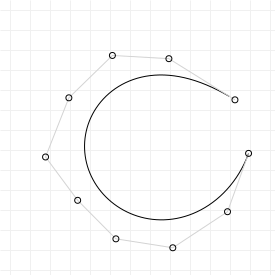
此即用n次曲线逼近n+1次曲线的表达式。这虽然不是精确拟合,但却是非常好的近似。下图对一条(半)随机的曲线实现了这些升次和降次的规则,图上的控制点可以移动,点击按钮可以升高或降低曲线的次数。
导数
利用贝塞尔函数的导数可以对贝塞尔曲线做一些有用的事,而贝塞尔函数较为有趣的一个性质是其导数也为贝塞尔函数。其实贝塞尔函数的求导相对而言比较直接,只是需要一点数学运算。
首先观察贝塞尔函数的求导法则,即:

上式可改写为(注意式中的b即权重w,且n乘以一个和式等于每个求和项乘以n再求和):

直白地说,n次贝塞尔函数的导数为n-1次贝塞尔函数,少了一项,而且新的权重w'0、……、w'n-1可用旧的权重通过n(wi+1 - wi)求得。对于带四个权重的三次函数,其导数的三个新权重为:w'0 = 3(w1-w0),w'1 = 3(w2-w1)和w'2 = 3(w3-w2)。
“慢着,为什么这是对的?”
虽然有时候有人告诉说“这是导数”就行,但还是可能想一探究竟。既然如此,就来看看这个导数的证明。首先,因为权重不影响完整的贝塞尔函数的求导,所以求导只涉及多项式基函数的导数。基函数的导数为:


上式不易处理,因此打开括号:

现在技巧性的一步是将上式再次化为含二项式系数的形式,需要得到形如“x!/y!(x-y)!”的项。如果得到关于n-1和k-1的项,那么说明方向是对的。

这是第一步。上式括号里的两项其实为标准的、低一次的贝塞尔函数:

现在将上式应用于已有的加权贝塞尔函数。先写出之前所见的平面曲线公式,再逐步求出导数:

如果打开上式的括号(用颜色表示相匹配的项),再按递增的k值重排各项,那么有:

上式中有两项会消失掉:因为任意和式都没有第-1项,所以上式第一项消失。既然这一项总是贡献为零,那么求导时就可以放心地将其完全无视。消失的另外一项为展开式的最后一项——包含Bn-1,n的一项。这一项含有二项式系数Cii+1,而这一系数通常约定等于0。因此这一项贡献为零,也可被略去。这意味着剩下的项为:

此即低次函数之和:

将上式改写为正常的和式即可:

将上式改写为与原式相似的形式有助于看出它们的区别。先写出原式,再写出导数:


有什么区别?对于实际的贝塞尔曲线而言几乎没有区别!虽然次数降低了(从n次变为n-1次),但是贝塞尔函数没有改变。唯一的真正的区别在于推导表示曲线的函数时权重如何变化。如果有A、B、C、D四个点,那么导数有三个点,二阶导数有两个点,三阶导数有一个点:

只要有多于一个权重即可运用这一方法。只剩一个权重时,下一步会出现k=0,而贝塞尔函数的和式因为无项可加而化为零。因此二次函数没有二阶导数,三次函数没有三阶导数,更一般地有n次函数有n-1阶(有意义的)导数,其更高阶导数为零。
切线与法线
如果要将物体沿曲线移动或者从曲线附近“移向远处”,那么与之最相关的两个向量为曲线的切向量和法向量,而这两者都非常容易求得。切向量用于沿曲线移动或者对准曲线方向,它标志着曲线在指定点的行进方向,而且就是曲线函数的一阶导数:

此即所需的方向向量。可以在每一点将方向向量规范化后得到单位方向向量(即长度为1.0),再根据这些方向进行所需的操作:

切向量对于沿曲线移动很有用,但如果要从曲线附近“移向远处”,而且移动方向与曲线在某点t处垂直,那该怎么办?这时需要的是法向量。这一向量与曲线的方向保持垂直,且长度通常为1.0,因此只需旋转单位方向向量即可:

其实旋转坐标只要知道方法就非常简单——“施加旋转矩阵”,以下即采用这种方法。本质上这一做法是先选取用于旋转的圆,再将坐标沿着圆“滑动所需的角度”。如果需要转动90度,那么将坐标沿着圆滑动90度即可。
为了将点(x,y)(绕(0,0))旋转φ度得到点(x',y'),可以使用以下简洁的计算式:

对应“短”版本的矩阵变换为:

注意对于90度、180度和270度旋转,因为这些角度的正弦和余弦分别为0和1、-1和0、0和-1,所以上式可以更简。
但是**为什么**可以这样做?为什么用这一矩阵乘法?这是因为旋转变换可以表示为三个(初等)剪切变换的复合,而将三个变换合成一个变换(因为所有矩阵变换都可以复合)即得上述矩阵表示。DataGenetics对此进行了很好的解释,非常推荐读者一读。
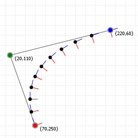
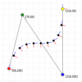
以下两图展示了二次和三次贝塞尔曲线在各点的切线和法线,其中蓝色的为方向向量,红色的为法向量(标记按t值的等分区间放置,并非等距放置)。
三维法向量
在进入下一章之前需要花点时间探究二维和三维的区别。尽管这一区别影响的范围不大无关且两种情形的做法相同(比如求三维切向量与二维情形所做的一样,不过所求为x、y、z而不只是x、y),但是法向量的情况有点复杂,所做的也就更多。尽管不是“极其困难”,但是所需的步骤更多,需要仔细看看。
三维法向量的求法原则上与二维一样——将规范化的切向量旋转90度。然而这就是情况变得略微复杂的地方:因为三维的“法向量”是法平面上的任意一个向量,所以可以旋转的方向并不唯一,因此需要定义三维情形中“唯一的”法向量是什么。
“朴素”的方法是构造弗勒内法向量,而以下采用的简单做法在很多情况下都可行(但在其他情况下会得到极其怪异的结果)。思路是虽然有无穷多个向量与切向量垂直(即与之成90度角),但是切向量本身已差不多位于自带的平面上——因为曲线上的每一点(无论间隔多小)都有自己的切向量,所以可以说每个点都位于此处的切向量和“近旁”的切向量所在的平面上。
即使这两个切向量的差微乎其微,只要“有差”就可求出这一平面,或者说求出垂直于平面的向量。计算出这一向量之后,因为切向量在平面上,所以将切向量绕垂直向量旋转即可。计算这一法向量的逻辑与二维情形相同——“直接旋转90度”。
那么开始吧!令人意外的是四行就做完了:
- a = normalize(B'(t))
- b = normalize(a + B''(t))
- r = normalize(b × a)
- normal = normalize(r × a)
展开说几句:
- 先将曲线上一点的导数规范化得到单位向量。规范化可以减少计算量,而计算量越少越好。
- 再计算b。假如曲线从这个点开始不再变化,保持导数和二阶导数不变,则b表示下一个点处的切向量。
- 得到两个共面向量后(导数、导数与二阶导数的和),用叉积这一基本的向量运算可以求出与这一平面垂直的向量。(注意这一运算使用的符号×绝非乘法运算!)叉积所得向量可以当做“旋转轴”,像二维情形一样将切向量旋转90度得到法向量。
- 既然由叉积可得垂直于由两个向量所确定的平面的另一向量,而法向量又与切向量和旋转轴所在平面垂直,那么再用一次叉积即得法向量。
这样就求出了三维曲线“唯一”的法向量。以一条曲线为例看看效果如何?从左往右拖动滚动条,根据鼠标位置所确定的t值显示在此处的法向量——最左为0,最右为1,中间为0.5,等等:
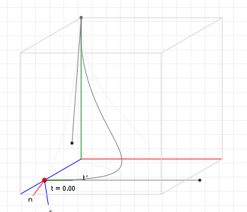
然而摆弄图像一阵之后可能会察觉到异样——法向量似乎在t=0.65和t=0.75之间“绕着曲线急转弯”……为什么会这样?
其实出现这种现象是因为数学公式就是这样推导的,所以弗勒内法向量的问题就在于此:虽然“从数学上看”是对的,但是“从实际上看”有问题。因此为了让任何图像都不出问题,所真正需要的是只要……看起来不错就好的方法。
还好不只有弗勒内法向量这一种选择。另一种选择是采用稍微偏算法的方式计算一种形式的旋转最小化标架(亦称“平行输运标架”或“比舍标架”),此处“标架”是以线上点为原点,由切向量、旋转轴和法向量构成的集合。
因为计算这种类型的标架依赖于“上一个标架”,所以无法像弗勒内标架一样“按需”对单独的点直接计算,而是需要对整条曲线进行计算。好在计算过程相当简单,而且可以与曲线查询表的构建同时进行。
思路是在t=0处取一个由切向量、旋转轴、法向量构成的初始标架,再使用一定的规则计算下一标架“应有”的形式。上文链接的旋转最小化标架论文给出的规则为:
- 取曲线上已经求出旋转最小化标架的一个点,
- 取曲线上尚未求出旋转最小化标架的下一个点,
- 再以上一个点和下一个点的中垂面为镜面,将已有标架翻转到下一个点上。
- 翻转后的切向量方向与下一个点的切向量方向大致相反,而且法向量也略有歪斜。
- 于是再以翻转后的切向量和下一个点的切向量所确定的平面为镜面,将翻转后的标架再次翻转。
- 切向量和法向量修正完毕,所得即为好用的标架。
来写点代码吧!
实现旋转最小化标架
首先假设已有函数用于计算上文提及的指定点的弗勒内标架,输出的标架具有如下性质:
{
  o:所有向量的起点,即线上点;
  t:切向量;
  r:旋转轴向量;
  n:法向量
}
再如下写出生成一系列旋转最小化标架的函数:
generateRMFrames(steps) -> frames:
  step = 1.0/steps
  // 从曲线上t=0处标准的切向量/旋转轴/法向量标架开始:
  frames.add(getFrenetFrame(0))
  // 开始构造旋转最小化标架:
  for t0 = 0, t0 < 1.0, t0 += step:
    // 从已有的上一标架开始
    x0 = frames.last
    // 求出下一标架:要保留它的位置和切向量,
    // 但要重新计算轴向量和法向量。
    t1 = t0 + step
    x1 = { o: getPoint(t1), t: getDerivative(t) }
    // 首先以x0和x1的中垂面为镜面,
    // 将x0的切向量和旋转轴翻转到x1处
    v1 = x1.o - x0.o
    c1 = v1 · v1
    riL = x0.r - v1 * 2/c1 * v1 · x0.r
    tiL = x0.t - v1 * 2/c1 * v1 · x0.t
    // 注意到v1为向量,而2/c1和v1 · ……就是数,
    // 因此上述代码只是对v1进行一定倍数的缩放。
    // 然后再以过x1的平面为镜面再次翻转,
    // 标架向量的方向即重新与曲线切向量一致:
    v2 = x1.t - tiL
    c2 = v2 · v2
    // 收尾工作:
    x1.r = riL - v2 * 2/c2 * v2 · riL
    x1.n = x1.r × x1.t
    frames.add(x1)
即使忽略注释,代码也明显比计算单个弗勒内标架的多,但也没有多得离谱,而且得到了长得更好的法向量。
提到长得更好,这样的标架到底是什么样子?下面回顾之前的那条曲线,但这次用的不是弗勒内标架而是旋转最小化标架:
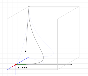
看起来好多了!
给看过代码的读者的话:严格来说一开始甚至不需要弗勒内标架。比方说可以将z轴当作初始旋转轴,于是初始法向量为 (0,0,1) × 切向量,然后再继续下去。不过求出“数学上正确”的初始标架,从而让初始法向量的方向符合曲线在三维空间中的定向,这总归是不错的。
分量函数
当人们开始在自己的程序中使用贝塞尔曲线时,首先遇到的问题之一是:“我虽然知道怎么画曲线,但是怎么确定包围盒?”其实做法颇为直接,但需要知道如何利用一些数学知识得到所需的值。对于包围盒而言,所需的其实并不是曲线本身,而只是曲线的“极值”——曲线的x轴和y轴分量的最小值和最大值。如果还记得微积分的话(前提是学过微积分,否则更难记),那么函数的极值可以用函数的一阶导数所确定,但由于“曲线函数”有不只一个分量,这就产生了一个问题——每个分量都有自己的函数。
解决办法:对每个分量分别计算导数,再按照原来的分量顺序重新拼在一起。
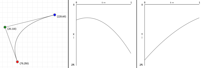
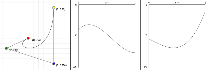
以下演示参数化的贝塞尔曲线如何“分解”为两个正常的函数,一个对应于x轴,一个对应于y轴。注意左侧的图像依然是可交互的曲线,但没有标出坐标轴(坐标显示在图中);中间和右侧的图像是分量函数,分别对应于指定t值(介于0和1之间,含端点)后求出的x轴和y轴分量。
如果水平移动曲线上的点,那么应当只有中间的图像在变化;同样,如果竖直移动曲线上的点,那么应当只有右侧的图像在变化。
Finding extremities: root finding
Now that we understand (well, superficially anyway) the component functions, we can find the extremities of our Bézier curve by finding maxima and minima on the component functions, by solving the equation B'(t) = 0. We've already seen that the derivative of a Bézier curve is a simpler Bézier curve, but how do we solve the equality? Fairly easily, actually, until our derivatives are 4th order or higher... then things get really hard. But let's start simple:
Quadratic curves: linear derivatives.
The derivative of a quadratic Bézier curve is a linear Bézier curve, interpolating between just two terms, which means finding the
solution for "where is this line 0" is effectively trivial by rewriting it to a function of t and solving. First we turn our
quadratic Bézier function into a linear one, by following the rule mentioned at the end of the
derivatives section:

And then we turn this into our solution for t using basic arithmetics:

Done.
Although with the caveat that if b-a is zero, there
is no solution and we probably shouldn't try to perform that division.
Cubic curves: the quadratic formula.
The derivative of a cubic Bézier curve is a quadratic Bézier curve, and finding the roots for a quadratic polynomial means we can apply the Quadratic formula. If you've seen it before, you'll remember it, and if you haven't, it looks like this:

So, if we can rewrite the Bézier component function as a plain polynomial, we're done: we just plug in the values into the quadratic formula, check if that square root is negative or not (if it is, there are no roots) and then just compute the two values that come out (because of that plus/minus sign we get two). Any value between 0 and 1 is a root that matters for Bézier curves, anything below or above that is irrelevant (because Bézier curves are only defined over the interval [0,1]). So, how do we convert?
First we turn our cubic Bézier function into a quadratic one, by following the rule mentioned at the end of the derivatives section:

And then, using these v values, we can find out what our a, b, and c should be:

This gives us three coefficients {a, b, c} that are expressed in terms of v values, where the v values are
expressions of our original coordinate values, so we can do some substitution to get:

Easy-peasy. We can now almost trivially find the roots by plugging those values into the quadratic formula.
And as a cubic curve, there is also a meaningful second derivative, which we can compute by simple taking the derivative of the derivative.
Quartic curves: Cardano's algorithm.
We haven't really looked at them before now, but the next step up would be a Quartic curve, a fourth degree Bézier curve. As expected, these have a derivative that is a cubic function, and now things get much harder. Cubic functions don't have a "simple" rule to find their roots, like the quadratic formula, and instead require quite a bit of rewriting to a form that we can even start to try to solve.
Back in the 16th century, before Bézier curves were a thing, and even before calculus itself was a thing, Gerolamo Cardano figured out that even if the general cubic function is really hard to solve, it can be rewritten to a form for which finding the roots is "easier" (even if not "easy"):

We can see that the easier formula only has two constants, rather than four, and only two expressions involving t, rather
than three: this makes things considerably easier to solve because it lets us use
regular calculus to find the values that satisfy the equation.
Now, there is one small hitch: as a cubic function, the solutions may be complex numbers rather than plain numbers... And Cardano realised this, centuries before complex numbers were a well-understood and established part of number theory. His interpretation of them was "these numbers are impossible but that's okay because they disappear again in later steps", allowing him to not think about them too much, but we have it even easier: as we're trying to find the roots for display purposes, we don't even care about complex numbers: we're going to simplify Cardano's approach just that tiny bit further by throwing away any solution that's not a plain number.
So, how do we rewrite the hard formula into the easier formula? This is explained in detail over at Ken J. Ward's page for solving the cubic equation, so instead of showing the maths, I'm simply going to show the programming code for solving the cubic equation, with the complex roots getting totally ignored, but if you're interested you should definitely head over to Ken's page and give the procedure a read-through.
Implementing Cardano's algorithm for finding all real roots
The "real roots" part is fairly important, because while you cannot take a square, cube, etc. root of a negative number in the "real" number space (denoted with ℝ), this is perfectly fine in the "complex" number space (denoted with ℂ). And, as it so happens, Cardano is also attributed as the first mathematician in history to have made use of complex numbers in his calculations. For this very algorithm!
| 1 | |
| 2 | |
| 3 | |
| 4 | |
| 5 | |
| 6 | |
| 7 | |
| 8 | |
| 9 | |
| 10 | |
| 11 | |
| 12 | |
| 13 | |
| 14 | |
| 15 | |
| 16 | |
| 17 | |
| 18 | |
| 19 | |
| 20 | |
| 21 | |
| 22 | |
| 23 | |
| 24 | |
| 25 | |
| 26 | |
| 27 | |
| 28 | |
| 29 | |
| 30 | |
| 31 | |
| 32 | |
| 33 | |
| 34 | |
| 35 | |
| 36 | |
| 37 | |
| 38 | |
| 39 | |
| 40 | |
| 41 | |
| 42 | |
| 43 | |
| 44 | |
| 45 | |
| 46 | |
| 47 | |
| 48 | |
| 49 | |
| 50 | |
| 51 | |
| 52 | |
| 53 | |
| 54 | |
| 55 | |
| 56 | |
| 57 | |
| 58 | |
| 59 | |
| 60 | |
| 61 | |
| 62 | |
| 63 | |
| 64 | |
| 65 | |
| 66 | |
| 67 | |
| 68 | |
| 69 | |
| 70 | |
| 71 | |
| 72 | |
| 73 | |
| 74 | |
| 75 | |
| 76 | |
| 77 | |
| 78 | |
| 79 | |
| 80 | |
| 81 |
And that's it. The maths is complicated, but the code is pretty much just "follow the maths, while caching as many values as we can to prevent recomputing things as much as possible" and now we have a way to find all roots for a cubic function and can just move on with using that to find extremities of our curves.
And of course, as a quartic curve also has meaningful second and third derivatives, we can quite easily compute those by using the derivative of the derivative (of the derivative), just as for cubic curves.
Quintic and higher order curves: finding numerical solutions
And this is where thing stop, because we cannot find the roots for polynomials of degree 5 or higher using algebra (a fact known as the Abel–Ruffini theorem). Instead, for occasions like these, where algebra simply cannot yield an answer, we turn to numerical analysis.
That's a fancy term for saying "rather than trying to find exact answers by manipulating symbols, find approximate answers by describing the underlying process as a combination of steps, each of which can be assigned a number via symbolic manipulation". For example, trying to mathematically compute how much water fits in a completely crazy three dimensional shape is very hard, even if it got you the perfect, precise answer. A much easier approach, which would be less perfect but still entirely useful, would be to just grab a buck and start filling the shape until it was full: just count the number of buckets of water you used. And if we want a more precise answer, we can use smaller buckets.
So that's what we're going to do here, too: we're going to treat the problem as a sequence of steps, and the smaller we can make each
step, the closer we'll get to that "perfect, precise" answer. And as it turns out, there is a really nice numerical root-finding
algorithm, called the Newton-Raphson root finding method (yes, after
that Newton), which we can make use of. The Newton-Raphson approach
consists of taking our impossible-to-solve function f(x), picking some initial value x (literally any value will
do), and calculating f(x). We can think of that value as the "height" of the function at x. If that height is
zero, we're done, we have found a root. If it isn't, we calculate the tangent line at f(x) and calculate at which
x value its height is zero (which we've already seen is very easy). That will give us a new x and we
repeat the process until we find a root.
Mathematically, this means that for some x, at step n=1, we perform the following calculation until
fy(x) is zero, so that the next t is the same as the one we already have:

(The Wikipedia article has a decent animation for this process, so I will not add a graphic for that here)
Now, this works well only if we can pick good starting points, and our curve is continuously differentiable and doesn't have oscillations. Glossing over the exact meaning of those terms, the curves we're dealing with conform to those constraints, so as long as we pick good starting points, this will work. So the question is: which starting points do we pick?
As it turns out, Newton-Raphson is so blindingly fast that we could get away with just not picking: we simply run the algorithm from t=0 to t=1 at small steps (say, 1/200th) and the result will be all the roots we want. Of course, this may pose problems for high order Bézier curves: 200 steps for a 200th order Bézier curve is going to go wrong, but that's okay: there is no reason (at least, none that I know of) to ever use Bézier curves of crazy high orders. You might use a fifth order curve to get the "nicest still remotely workable" approximation of a full circle with a single Bézier curve, but that's pretty much as high as you'll ever need to go.
In conclusion:
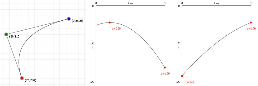
So now that we know how to do root finding, we can determine the first and second derivative roots for our Bézier curves, and show those roots overlaid on the previous graphics. For the quadratic curve, that means just the first derivative, in red:
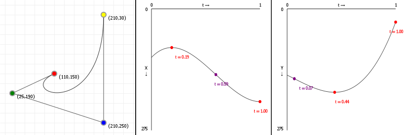
And for cubic curves, that means first and second derivatives, in red and purple respectively:
Bounding boxes
If we have the extremities, and the start/end points, a simple for-loop that tests for min/max values for x and y means we have the four values we need to box in our curve:
Computing the bounding box for a Bézier curve:
- Find all t value(s) for the curve derivative's x- and y-roots.
- Discard any t value that's lower than 0 or higher than 1, because Bézier curves only use the interval [0,1].
- Determine the lowest and highest value when plugging the values t=0, t=1 and each of the found roots into the original functions: the lowest value is the lower bound, and the highest value is the upper bound for the bounding box we want to construct.
Applying this approach to our previous root finding, we get the following axis-aligned bounding boxes (with all curve extremity points shown on the curve):
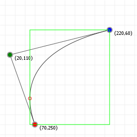
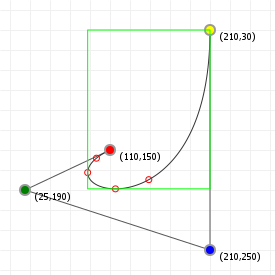
We can construct even nicer boxes by aligning them along our curve, rather than along the x- and y-axis, but in order to do so we first need to look at how aligning works.
Aligning curves
While there are an incredible number of curves we can define by varying the x- and y-coordinates for the control points, not all curves are actually distinct. For instance, if we define a curve, and then rotate it 90 degrees, it's still the same curve, and we'll find its extremities in the same spots, just at different draw coordinates. As such, one way to make sure we're working with a "unique" curve is to "axis-align" it.
Aligning also simplifies a curve's functions. We can translate (move) the curve so that the first point lies on (0,0), which turns our n term polynomial functions into n-1 term functions. The order stays the same, but we have less terms. Then, we can rotate the curves so that the last point always lies on the x-axis, too, making its coordinate (...,0). This further simplifies the function for the y-component to an n-2 term function. For instance, if we have a cubic curve such as this:

Then translating it so that the first coordinate lies on (0,0), moving all x coordinates by -120, and all y coordinates by -160, gives us:

If we then rotate the curve so that its end point lies on the x-axis, the coordinates (integer-rounded for illustrative purposes here) become:

If we drop all the zero-terms, this gives us:

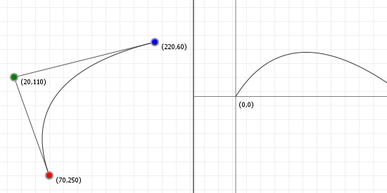
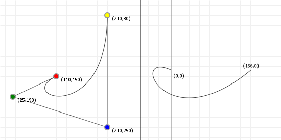
We can see that our original curve definition has been simplified considerably. The following graphics illustrate the result of aligning our example curves to the x-axis, with the cubic case using the coordinates that were just used in the example formulae:
Tight bounding boxes
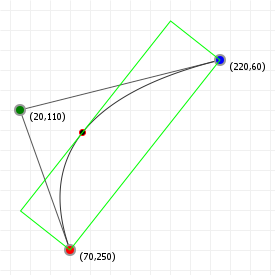
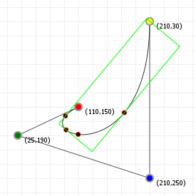
With our knowledge of bounding boxes, and curve alignment, We can now form the "tight" bounding box for curves. We first align our curve, recording the translation we performed, "T", and the rotation angle we used, "R". We then determine the aligned curve's normal bounding box. Once we have that, we can map that bounding box back to our original curve by rotating it by -R, and then translating it by -T.
We now have nice tight bounding boxes for our curves:
These are, strictly speaking, not necessarily the tightest possible bounding boxes. It is possible to compute the optimal bounding box by determining which spanning lines we need to effect a minimal box area, but because of the parametric nature of Bézier curves this is actually a rather costly operation, and the gain in bounding precision is often not worth it.
Curve inflections
Now that we know how to align a curve, there's one more thing we can calculate: inflection points. Imagine we have a variable size circle that we can slide up against our curve. We place it against the curve and adjust its radius so that where it touches the curve, the curvatures of the curve and the circle are the same, and then we start to slide the circle along the curve - for quadratic curves, we can always do this without the circle behaving oddly: we might have to change the radius of the circle as we slide it along, but it'll always sit against the same side of the curve.
But what happens with cubic curves? Imagine we have an S curve and we place our circle at the start of the curve, and start sliding it along. For a while we can simply adjust the radius and things will be fine, but once we get to the midpoint of that S, something odd happens: the circle "flips" from one side of the curve to the other side, in order for the curvatures to keep matching. This is called an inflection, and we can find out where those happen relatively easily.
What we need to do is solve a simple equation:

What we're saying here is that given the curvature function C(t), we want to know for which values of t this function is zero, meaning there is no "curvature", which will be exactly at the point between our circle being on one side of the curve, and our circle being on the other side of the curve. So what does C(t) look like? Actually something that seems not too hard:

The function C(t) is the cross product between the first and second derivative functions for the parametric dimensions of our curve. And, as already shown, derivatives of Bézier curves are just simpler Bézier curves, with very easy to compute new coefficients, so this should be pretty easy.
However as we've seen in the section on aligning, aligning lets us simplify things a lot, by completely removing the contributions of the first coordinate from most mathematical evaluations, and removing the last y coordinate as well by virtue of the last point lying on the x-axis. So, while we can evaluate C(t) = 0 for our curve, it'll be much easier to first axis-align the curve and then evaluating the curvature function.
Let's derive the full formula anyway
Of course, before we do our aligned check, let's see what happens if we compute the curvature function without axis-aligning. We start with the first and second derivatives, given our basis functions:

And of course the same functions for y:

Asking a computer to now compose the C(t) function for us (and to expand it to a readable form of simple terms) gives us this rather overly complicated set of arithmetic expressions:

That is... unwieldy. So, we note that there are a lot of terms that involve multiplications involving x1, y1, and y4, which would all disappear if we axis-align our curve, which is why aligning is a great idea.
Aligning our curve so that three of the eight coefficients become zero, and observing that scale does not affect finding
t values, we end up with the following simple term function for C(t):

That's a lot easier to work with: we see a fair number of terms that we can compute and then cache, giving us the following simplification:

This is a plain quadratic curve, and we know how to solve C(t) = 0; we use the quadratic formula:

We can easily compute this value if the discriminator isn't a negative number (because we only want real roots, not complex roots), and if x is not zero, because divisions by zero are rather useless.
Taking that into account, we compute t, we disregard any t value that isn't in the Bézier interval [0,1], and we now know at which t value(s) our curve will inflect.
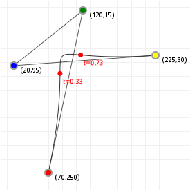
The canonical form (for cubic curves)
While quadratic curves are relatively simple curves to analyze, the same cannot be said of the cubic curve. As a curvature is controlled by more than one control point, it exhibits all kinds of features like loops, cusps, odd colinear features, and as many as two inflection points because the curvature can change direction up to three times. Now, knowing what kind of curve we're dealing with means that some algorithms can be run more efficiently than if we have to implement them as generic solvers, so is there a way to determine the curve type without lots of work?
As it so happens, the answer is yes, and the solution we're going to look at was presented by Maureen C. Stone from Xerox PARC and Tony D. deRose from the University of Washington in their joint paper "A Geometric Characterization of Parametric Cubic curves". It was published in 1989, and defines curves as having a "canonical" form (i.e. a form that all curves can be reduced to) from which we can immediately tell what features a curve will have. So how does it work?
The first observation that makes things work is that if we have a cubic curve with four points, we can apply a linear transformation to these points such that three of the points end up on (0,0), (0,1) and (1,1), with the last point then being "somewhere". After applying that transformation, the location of that last point can then tell us what kind of curve we're dealing with. Specifically, we see the following breakdown:
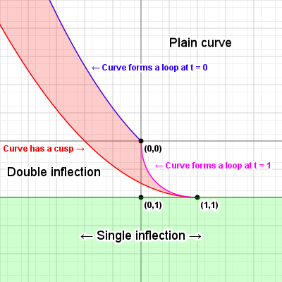
This is a fairly funky image, so let's see what the various parts of it mean...
We see the three fixed points at (0,0), (0,1) and (1,1). The various regions and boundaries indicate what property the original curve will have, if the fourth point is in/on that region or boundary. Specifically, if the fourth point is...
-
...anywhere inside the red zone, but not on its boundaries, the curve will be self-intersecting (yielding a loop). We won't know where it self-intersects (in terms of t values), but we are guaranteed that it does.
-
...on the left (red) edge of the red zone, the curve will have a cusp. We again don't know where, but we know there is one. This edge is described by the function:
-
...on the almost circular, lower right (pink) edge, the curve's end point touches the curve, forming a loop. This edge is described by the function:
-
...on the top (blue) edge, the curve's start point touches the curve, forming a loop. This edge is described by the function:
-
...inside the lower (green) zone, past
y=1, the curve will have a single inflection (switching concave/convex once). -
...between the left and lower boundaries (below the cusp line but above the single-inflection line), the curve will have two inflections (switching from concave to convex and then back again, or from convex to concave and then back again).
...anywhere on the right of self-intersection zone, the curve will have no inflections. It'll just be a simple arch.
Of course, this map is fairly small, but the regions extend to infinity, with well defined boundaries.
Wait, where do those lines come from?
Without repeating the paper mentioned at the top of this section, the loop-boundaries come from rewriting the curve into canonical form, and then solving the formulae for which constraints must hold for which possible curve properties. In the paper these functions yield formulae for where you will find cusp points, or loops where we know t=0 or t=1, but those functions are derived for the full cubic expression, meaning they apply to t=-∞ to t=∞... For Bézier curves we only care about the "clipped interval" t=0 to t=1, so some of the properties that apply when you look at the curve over an infinite interval simply don't apply to the Bézier curve interval.
The right bound for the loop region, indicating where the curve switches from "having inflections" to "having a loop", for the general cubic curve, is actually mirrored over x=1, but for Bézier curves this right half doesn't apply, so we don't need to pay attention to it. Similarly, the boundaries for t=0 and t=1 loops are also nice clean curves but get "cut off" when we only look at what the general curve does over the interval t=0 to t=1.
For the full details, head over to the paper and read through sections 3 and 4. If you still remember your high school pre-calculus, you can probably follow along with this paper, although you might have to read it a few times before all the bits "click".
So now the question becomes: how do we manipulate our curve so that it fits this canonical form, with three fixed points, and one "free" point? Enter linear algebra. Don't worry, I'll be doing all the math for you, as well as show you what the effect is on our curves, but basically we're going to be using linear algebra, rather than calculus, because "it's way easier". Sometimes a calculus approach is very hard to work with, when the equivalent geometrical solution is super obvious.
The approach is going to start with a curve that doesn't have all-colinear points (so we need to make sure the points don't all fall on a straight line), and then applying three graphics operations that you will probably have heard of: translation (moving all points by some fixed x- and y-distance), scaling (multiplying all points by some x and y scale factor), and shearing (an operation that turns rectangles into parallelograms).
Step 1: we translate any curve by -p1.x and -p1.y, so that the curve starts at (0,0). We're going to make use of an interesting trick here, by pretending our 2D coordinates are 3D, with the z coordinate simply always being 1. This is an old trick in graphics to overcome the limitations of 2D transformations: without it, we can only turn (x,y) coordinates into new coordinates of the form (ax + by, cx + dy), which means we can't do translation, since that requires we end up with some kind of (x + a, y + b). If we add a bogus z coordinate that is always 1, then we can suddenly add arbitrary values. For example:

Sweet! z stays 1, so we can effectively ignore it entirely, but we added some plain values to our x and y coordinates. So, if we want to subtract p1.x and p1.y, we use:

Running all our coordinates through this transformation gives a new set of coordinates, let's call those U, where the first coordinate lies on (0,0), and the rest is still somewhat free. Our next job is to make sure point 2 ends up lying on the x=0 line, so what we want is a transformation matrix that, when we run it, subtracts x from whatever x we currently have. This is called shearing, and the typical x-shear matrix and its transformation looks like this:

So we want some shearing value that, when multiplied by y, yields -x, so our x coordinate becomes zero. That value is simply -x/y, because -x/y \ y = -x*. Done:

Now, running this on all our points generates a new set of coordinates, let's call those V, which now have point 1 on (0,0) and point 2 on (0, some-value), and we wanted it at (0,1), so we need to do some scaling to make sure it ends up at (0,1). Additionally, we want point 3 to end up on (1,1), so we can also scale x to make sure its x-coordinate will be 1 after we run the transform. That means we'll be x-scaling by 1/point3x, and y-scaling by point2y. This is really easy:

Then, finally, this generates a new set of coordinates, let's call those W, of which point 1 lies on (0,0), point 2 lies on (0,1), and
point three lies on (1, ...) so all that's left is to make sure point 3 ends up at (1,1) - but we can't scale! Point 2 is already in the
right place, and y-scaling would move it out of (0,1) again, so our only option is to y-shear point three, just like how we x-sheared
point 2 earlier. In this case, we do the same trick, but with y/x rather than x/y because we're not x-shearing
but y-shearing. Additionally, we don't actually want to end up at zero (which is what we did before) so we need to shear towards an
offset, in this case 1:

And this generates our final set of four coordinates. Of these, we already know that points 1 through 3 are (0,0), (0,1) and (1,1), and only the last coordinate is "free". In fact, given any four starting coordinates, the resulting "transformation mapped" coordinate will be:

Okay, well, that looks plain ridiculous, but: notice that every coordinate value is being offset by the initial translation, and also notice that a lot of terms in that expression are repeated. Even though the maths looks crazy as a single expression, we can just pull this apart a little and end up with an easy-to-calculate bit of code!
First, let's just do that translation step as a "preprocessing" operation so we don't have to subtract the values all the time. What does that leave?

Suddenly things look a lot simpler: the mapped x is fairly straight forward to compute, and we see that the mapped y actually contains the mapped x in its entirety, so we'll have that part already available when we need to evaluate it. In fact, let's pull out all those common factors to see just how simple this is:

That's kind of super-simple to write out in code, I think you'll agree. Coding math tends to be easier than the formulae initially make it look!
How do you track all that?
Doing maths can be a pain, so whenever possible, I like to make computers do the work for me. Especially for things like this, I simply use Mathematica. Tracking all this math by hand is insane, and we invented computers, literally, to do this for us. I have no reason to use pen and paper when I can write out what I want to do in a program, and have the program do the math for me. And real math, too, with symbols, not with numbers. In fact, here's the Mathematica notebook if you want to see how this works for yourself.
Now, I know, you're thinking "but Mathematica is super expensive!" and that's true, it's $344 for home use, up from $295 when I original wrote this, but it's also free when you buy a $35 raspberry pi. Obviously, I bought a raspberry pi, and I encourage you to do the same. With that, as long as you know what you want to do, Mathematica can just do it for you. And we don't have to be geniuses to work out what the maths looks like. That's what we have computers for.
So, let's write up a sketch that'll show us the canonical form for any curve drawn in blue, overlaid on our canonical map, so that we can immediately tell which features our curve must have, based on where the fourth coordinate is located on the map:
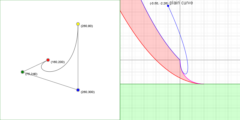
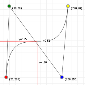
Finding Y, given X
One common task that pops up in things like CSS work, or parametric equalizers, or image leveling, or any other number of applications where Bézier curves are used as control curves in a way that there is really only ever one "y" value associated with one "x" value, you might want to cut out the middle man, as it were, and compute "y" directly based on "x". After all, the function looks simple enough, finding the "y" value should be simple too, right? Unfortunately, not really. However, it is possible and as long as you have some code in place to help, it's not a lot of a work either.
We'll be tackling this problem in two stages: the first, which is the hard part, is figuring out which "t" value belongs to any given "x"
value. For instance, have a look at the following graphic. On the left we have a Bézier curve that looks for all intents and purposes like
it fits our criteria: every "x" has one and only one associated "y" value. On the right we see the function for just the "x" values:
that's a cubic curve, but not a really crazy cubic curve. If you move the graphic's slider, you will see a red line drawn that corresponds
to the x coordinate: this is a vertical line in the left graphic, and a horizontal line on the right.
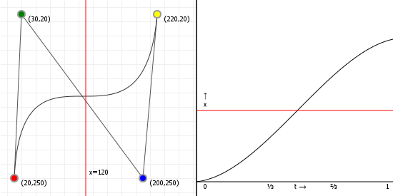
Now, if you look more closely at that right graphic, you'll notice something interesting: if we treat the red line as "the x axis", then the point where the function crosses our line is really just a root for the cubic function x(t) through a shifted "x-axis"... and we've already seen how to calculate roots, so let's just run cubic root finding - and not even the complicated cubic case either: because of the kind of curve we're starting with, we know there is at most a single root in the interval [0,1], simplifying the code we need!
First, let's look at the function for x(t):

We can rewrite this to a plain polynomial form, by just fully writing out the expansion and then collecting the polynomial factors, as:

Nothing special here: that's a standard cubic polynomial in "power" form (i.e. all the terms are ordered by their power of
t). So, given that a, b, c, d, and x(t) are all
known constants, we can trivially rewrite this (by moving the x(t) across the equal sign) as:

You might be wondering "where did all the other 'minus x' for all the other values a, b, c, and d go?" and the answer there is that they all cancel out, so the only one we actually need to subtract is the one at the end. Handy! So now we just solve this equation using Cardano's algorithm, and we're left with some rather short code:
| 1 | |
| 2 | |
| 3 | |
| 4 | |
| 5 | |
| 6 | |
| 7 | |
| 8 | |
| 9 | |
| 10 |
So the procedure is fairly straight forward: pick an x, find the associated t value, evaluate our curve
for that t value, which gives us the curve's {x,y} coordinate, which means we know y for this
x. Move the slider for the following graphic to see this in action:
Arc length
How long is a Bézier curve? As it turns out, that's not actually an easy question, because the answer requires maths that —much like root finding— cannot generally be solved the traditional way. If we have a parametric curve with fx(t) and fy(t), then the length of the curve, measured from start point to some point t = z, is computed using the following seemingly straight forward (if a bit overwhelming) formula:

or, more commonly written using Leibnitz notation as:

This formula says that the length of a parametric curve is in fact equal to the area underneath a function that looks a remarkable amount like Pythagoras' rule for computing the diagonal of a straight angled triangle. This sounds pretty simple, right? Sadly, it's far from simple... cutting straight to after the chase is over: for quadratic curves, this formula generates an unwieldy computation, and we're simply not going to implement things that way. For cubic Bézier curves, things get even more fun, because there is no "closed form" solution, meaning that due to the way calculus works, there is no generic formula that allows you to calculate the arc length. Let me just repeat this, because it's fairly crucial: for cubic and higher Bézier curves, there is no way to solve this function if you want to use it "for all possible coordinates".
Seriously: It cannot be done.
So we turn to numerical approaches again. The method we'll look at here is the Gauss quadrature. This approximation is a really neat trick, because for any nth degree polynomial it finds approximated values for an integral really efficiently. Explaining this procedure in length is way beyond the scope of this page, so if you're interested in finding out why it works, I can recommend the University of South Florida video lecture on the procedure, linked in this very paragraph. The general solution we're looking for is the following:

In plain text: an integral function can always be treated as the sum of an (infinite) number of (infinitely thin) rectangular strips sitting "under" the function's plotted graph. To illustrate this idea, the following graph shows the integral for a sinusoid function. The more strips we use (and of course the more we use, the thinner they get) the closer we get to the true area under the curve, and thus the better the approximation:
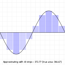
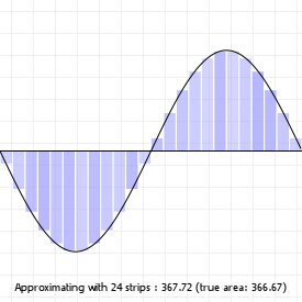
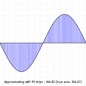
Now, infinitely many terms to sum and infinitely thin rectangles are not something that computers can work with, so instead we're going to approximate the infinite summation by using a sum of a finite number of "just thin" rectangular strips. As long as we use a high enough number of thin enough rectangular strips, this will give us an approximation that is pretty close to what the real value is.
So, the trick is to come up with useful rectangular strips. A naive way is to simply create n strips, all with the same width, but there is a far better way using special values for C and f(t) depending on the value of n, which indicates how many strips we'll use, and it's called the Legendre-Gauss quadrature.
This approach uses strips that are not spaced evenly, but instead spaces them in a special way based on describing the function as a polynomial (the more strips, the more accurate the polynomial), and then computing the exact integral for that polynomial. We're essentially performing arc length computation on a flattened curve, but flattening it based on the intervals dictated by the Legendre-Gauss solution.
Note that one requirement for the approach we'll use is that the integral must run from -1 to 1. That's no good, because we're dealing with Bézier curves, and the length of a section of curve applies to values which run from 0 to "some value smaller than or equal to 1" (let's call that value z). Thankfully, we can quite easily transform any integral interval to any other integral interval, by shifting and scaling the inputs. Doing so, we get the following:

That may look a bit more complicated, but the fraction involving z is a fixed number, so the summation, and the evaluation of the f(t) values are still pretty simple.
So, what do we need to perform this calculation? For one, we'll need an explicit formula for f(t), because that derivative notation is handy on paper, but not when we have to implement it. We'll also need to know what these Ci and ti values should be. Luckily, that's less work because there are actually many tables available that give these values, for any n, so if we want to approximate our integral with only two terms (which is a bit low, really) then these tables would tell us that for n=2 we must use the following values:

Which means that in order for us to approximate the integral, we must plug these values into the approximate function, which gives us:

We can program that pretty easily, provided we have that f(t) available, which we do, as we know the full description for the Bézier curve functions Bx(t) and By(t).
If we use the Legendre-Gauss values for our C values (thickness for each strip) and t values (location of each strip), we can determine the approximate length of a Bézier curve by computing the Legendre-Gauss sum. The following graphic shows a cubic curve, with its computed lengths; Go ahead and change the curve, to see how its length changes. One thing worth trying is to see if you can make a straight line, and see if the length matches what you'd expect. What if you form a line with the control points on the outside, and the start/end points on the inside?
Approximated arc length
Sometimes, we don't actually need the precision of a true arc length, and we can get away with simply computing the approximate arc length instead. The by far fastest way to do this is to flatten the curve and then simply calculate the linear distance from point to point. This will come with an error, but this can be made arbitrarily small by increasing the segment count.
If we combine the work done in the previous sections on curve flattening and arc length computation, we can implement these with minimal effort:
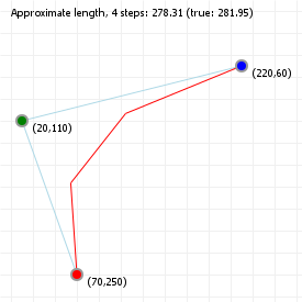

You may notice that even though the error in length is actually pretty significant in absolute terms, even at a low number of segments we get a length that agrees with the true length when it comes to just the integer part of the arc length. Quite often, approximations can drastically speed things up!
Curvature of a curve
If we have two curves, and we want to line them in up in a way that "looks right", what would we use as metric to let a computer decide what "looks right" means?
For instance, we can start by ensuring that the two curves share an end coordinate, so that there is no "gap" between the end of one and the start of the next curve, but that won't guarantee that things look right: both curves can be going in wildly different directions, and the resulting joined geometry will have a corner in it, rather than a smooth transition from one curve to the next.
What we want is to ensure that the curvature at the transition from one curve to the next "looks good". So, we start with a shared coordinate, and then also require that derivatives for both curves match at that coordinate. That way, we're assured that their tangents line up, which must mean the curve transition is perfectly smooth. We can even make the second, third, etc. derivatives match up for better and better transitions.
Problem solved!
However, there's a problem with this approach: if we think about this a little more, we realise that "what a curve looks like" and its derivative values are pretty much entirely unrelated. After all, the section on reordering curves showed us that the same looking curve can have an infinite number of curve expressions of arbitrarily high Bézier degree, and each of those will have wildly different derivative values.
So what we really want is some kind of expression that's not based on any particular expression of t, but is based on
something that is invariant to the kind of function(s) we use to draw our curve. And the prime candidate for this is our curve
expression, reparameterised for distance: no matter what order of Bézier curve we use, if we were able to rewrite it as a function of
distance-along-the-curve, all those different degree Bézier functions would end up being the same function for "coordinate at
some distance D along the curve".
We've seen this before... that's the arc length function.
So you might think that in order to find the curvature of a curve, we now need to solve the arc length function itself, and that this would be quite a problem because we just saw that there is no way to actually do that. Thankfully, we don't. We only need to know the form of the arc length function, which we saw above and is fairly simple, rather than needing to solve the arc length function. If we start with the arc length expression and the run through the steps necessary to determine its derivative (with an alternative, shorter demonstration of how to do this found over on Stackexchange), then the integral that was giving us so much problems in solving the arc length function disappears entirely (because of the fundamental theorem of calculus), and what we're left with us some surprisingly simple maths that relates curvature (denoted as κ, "kappa") to—and this is the truly surprising bit—a specific combination of derivatives of our original function.
Let me highlight what just happened, because it's pretty special:
- we wanted to make curves line up, and initially thought to match the curves' derivatives, but
- that turned out to be a really bad choice, so instead
- we picked a function that is basically impossible to work with, and then worked with that, which
- gives us a simple formula that is and expression using the curves' derivatives.
That's crazy!
But that's also one of the things that makes maths so powerful: even if your initial ideas are off the mark, you might be much closer than you thought you were, and the journey from "thinking we're completely wrong" to "actually being remarkably close to being right" is where we can find a lot of insight.
So, what does the function look like? This:

Which is really just a "short form" that glosses over the fact that we're dealing with functions of t, so let's expand that a
tiny bit:

And while that's a little more verbose, it's still just as simple to work with as the first function: the curvature at some point on any (and this cannot be overstated: any) curve is a ratio between the first and second derivative cross product, and something that looks oddly similar to the standard Euclidean distance function. And nothing in these functions is hard to calculate either: for Bézier curves, simply knowing our curve coordinates means we know what the first and second derivatives are, and so evaluating this function for any t value is just a matter of basic arithematics.
In fact, let's just implement it right now:
| 1 | |
| 2 | |
| 3 | |
| 4 | |
| 5 | |
| 6 | |
| 7 |
That was easy! (Well okay, that "not a number" value will need to be taken into account by downstream code, but that's a reality of programming anyway)
With all of that covered, let's line up some curves! The following graphic gives you two curves that look identical, but use quadratic and cubic functions, respectively. As you can see, despite their derivatives being necessarily different, their curvature (thanks to being derived based on maths that "ignores" specific function derivative, and instead gives a formula that smooths out any differences) is exactly the same. And because of that, we can put them together such that the point where they overlap has the same curvature for both curves, giving us the smoothest transition.
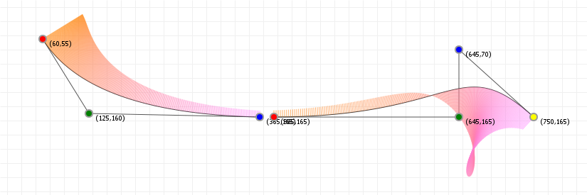
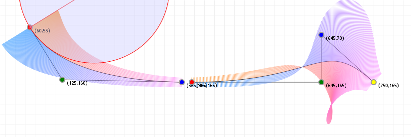
One thing you may have noticed in this sketch is that sometimes the curvature looks fine, but seems to be pointing in the wrong direction, making it hard to line up the curves properly. A way around that, of course, is to show the curvature on both sides of the curve, so let's just do that. But let's take it one step further: we can also compute the associated "radius of curvature", which gives us the implicit circle that "fits" the curve's curvature at any point, using what is possibly the simplest bit of maths found in this entire primer:

So let's revisit the previous graphic with the curvature visualised on both sides of our curves, as well as showing the circle that "fits" our curve at some point that we can control by using a slider:
Tracing a curve at fixed distance intervals
Say you want to draw a curve with a dashed line, rather than a solid line, or you want to move something along the curve at fixed distance intervals over time, like a train along a track, and you want to use Bézier curves.
Now you have a problem.
The reason you have a problem is that Bézier curves are parametric functions with non-linear behaviour, whereas moving a train along a
track is about as close to a practical example of linear behaviour as you can get. The problem we're faced with is that we can't just pick
t values at some fixed interval and expect the Bézier functions to generate points that are spaced a fixed distance apart. In
fact, let's look at the relation between "distance along a curve" and "t value", by plotting them against one another.
The following graphic shows a particularly illustrative curve, and its distance-for-t plot. For linear traversal, this line needs to be straight, running from (0,0) to (length,1). That is, it's safe to say, not what we'll see: we'll see something very wobbly, instead. To make matters even worse, the distance-for-t function is also of a much higher order than our curve is: while the curve we're using for this exercise is a cubic curve, which can switch concave/convex form twice at best, the distance function is our old friend the arc length function, which can have more inflection points.
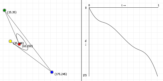
So, how do we "cut up" the arc length function at regular intervals, when we can't really work with it? We basically cheat: we run through
the curve using t values, determine the distance-for-this-t-value at each point we generate during the run, and
then we find "the closest t value that matches some required distance" using those values instead. If we have a low number of
points sampled, we can then even refine which t value "should" work for our desired distance by interpolating between two
points, but if we have a high enough number of samples, we don't even need to bother.
So let's do exactly that: the following graph is similar to the previous one, showing how we would have to "chop up" our distance-for-t
curve in order to get regularly spaced points on the curve. It also shows what using those t values on the real curve looks
like, by coloring each section of curve between two distance markers differently:
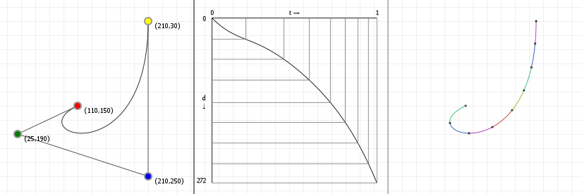
Use the slider to increase or decrease the number of equidistant segments used to colour the curve.
However, are there better ways? One such way is discussed in "Moving Along a Curve with Specified Speed" by David Eberly of Geometric Tools, LLC, but basically because we have no explicit length function (or rather, one we don't have to constantly compute for different intervals), you may simply be better off with a traditional lookup table (LUT).
Intersections
Let's look at some more things we will want to do with Bézier curves. Almost immediately after figuring out how to get bounding boxes to work, people tend to run into the problem that even though the minimal bounding box (based on rotation) is tight, it's not sufficient to perform true collision detection. It's a good first step to make sure there might be a collision (if there is no bounding box overlap, there can't be one), but in order to do real collision detection we need to know whether or not there's an intersection on the actual curve.
We'll do this in steps, because it's a bit of a journey to get to curve/curve intersection checking. First, let's start simple, by implementing a line-line intersection checker. While we can solve this the traditional calculus way (determine the functions for both lines, then compute the intersection by equating them and solving for two unknowns), linear algebra actually offers a nicer solution.
Line-line intersections
If we have two line segments with two coordinates each, segments A-B and C-D, we can find the intersection of the lines these segments are an intervals on by linear algebra, using the procedure outlined in this top coder article. Of course, we need to make sure that the intersection isn't just on the lines our line segments lie on, but actually on our line segments themselves. So after we find the intersection, we need to verify that it lies without the bounds of our original line segments.
The following graphic implements this intersection detection, showing a red point for an intersection on the lines our segments lie on (thus being a virtual intersection point), and a green point for an intersection that lies on both segments (being a real intersection point).
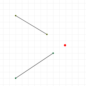
Implementing line-line intersections
Let's have a look at how to implement a line-line intersection checking function. The basics are covered in the article mentioned above, but sometimes you need more function signatures, because you might not want to call your function with eight distinct parameters. Maybe you're using point structs for the line. Let's get coding:
| 1 | |
| 2 | |
| 3 | |
| 4 | |
| 5 | |
| 6 | |
| 7 | |
| 8 | |
| 9 | |
| 10 | |
| 11 | |
| 12 | |
| 13 | |
| 14 | |
| 15 | |
| 16 | |
| 17 |
What about curve-line intersections?
Curve/line intersection is more work, but we've already seen the techniques we need to use in order to perform it: first we translate/rotate both the line and curve together, in such a way that the line coincides with the x-axis. This will position the curve in a way that makes it cross the line at points where its y-function is zero. By doing this, the problem of finding intersections between a curve and a line has now become the problem of performing root finding on our translated/rotated curve, as we already covered in the section on finding extremities.
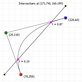
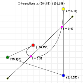
Curve/curve intersection, however, is more complicated. Since we have no straight line to align to, we can't simply align one of the curves and be left with a simple procedure. Instead, we'll need to apply two techniques we've met before: de Casteljau's algorithm, and curve splitting.
Curve/curve intersection
Using de Casteljau's algorithm to split the curve we can now implement curve/curve intersection finding using a "divide and conquer" technique:
- Take two curves C1 and C2, and treat them as a pair.
- If their bounding boxes overlap, split up each curve into two sub-curves
- With C1.1, C1.2, C2.1 and C2.2, form four new pairs (C1.1,C2.1), (C1.1, C2.2), (C1.2,C2.1), and (C1.2,C2.2).
-
For each pair, check whether their bounding boxes overlap.
- If their bounding boxes do not overlap, discard the pair, as there is no intersection between this pair of curves.
- If there is overlap, rerun all steps for this pair.
-
Once the sub-curves we form are so small that they effectively occupy sub-pixel areas, we consider an intersection found, noting that we
might have a cluster of multiple intersections at the sub-pixel level, out of which we pick one to act as "found"
tvalue (we can either throw all but one away, we can average the cluster'stvalues, or you can do something even more creative).
This algorithm will start with a single pair, "balloon" until it runs in parallel for a large number of potential sub-pairs, and then taper back down as it homes in on intersection coordinates, ending up with as many pairs as there are intersections.
The following graphic applies this algorithm to a pair of cubic curves, one step at a time, so you can see the algorithm in action. Click the button to run a single step in the algorithm, after setting up your curves in some creative arrangement. You can also change the value that is used in step 5 to determine whether the curves are small enough. Manipulating the curves or changing the threshold will reset the algorithm, so you can try this with lots of different curves.
(can you find the configuration that yields the maximum number of intersections between two cubic curves? Nine intersections!)
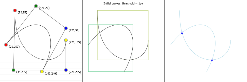
Finding self-intersections is effectively the same procedure, except that we're starting with a single curve, so we need to turn that into
two separate curves first. This is trivially achieved by splitting at an inflection point, or if there are none, just splitting at
t=0.5 first, and then running the exact same algorithm as above, with all non-overlapping curve pairs getting removed at each
iteration, and each successive step homing in on the curve's self-intersection points.
The projection identity
De Casteljau's algorithm is the pivotal algorithm when it comes to Bézier curves. You can use it not just to split curves, but also to draw them efficiently (especially for high-order Bézier curves), as well as to come up with curves based on three points and a tangent. Particularly this last thing is really useful because it lets us "mold" a curve, by picking it up at some point, and dragging that point around to change the curve's shape.
How does that work? Succinctly: we run de Casteljau's algorithm in reverse!
In order to run de Casteljau's algorithm in reverse, we need a few basic things: a start and end point, a point on the curve that we want to be moving around, which has an associated t value, and a point we've not explicitly talked about before, and as far as I know has no explicit name, but lives one iteration higher in the de Casteljau process then our on-curve point does. I like to call it "A" for reasons that will become obvious.
So let's use graphics instead of text to see where this "A" is, because text only gets us so far: move the sliders for the following
graphics to see what, given a specific t value, our A coordinate is. As well as some other coordinates, which
taken together let us derive a value that the graphics call "ratio": if you move the curve's points around, A, B, and C will move, what
happens to that value?
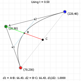
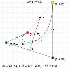
So these graphics show us several things:
- a point at the tip of the curve construction's "hat": let's call that
A, as well as - our on-curve point give our chosen
tvalue: let's call thatB, and finally, -
a point that we get by projecting A, through B, onto the line between the curve's start and end points: let's call that
C. -
for both quadratic and cubic curves, two points
e1ande2, which represent the single-to-last step in de Casteljau's algorithm: in the last step, we findBat(1-t) * e1 + t * e2. -
for cubic curves, also the points
v1andv2, which together withArepresent the first step in de Casteljau's algorithm: in the next step, we finde1ande2.
These three values A, B, and C allow us to derive an important identity formula for quadratic and cubic Bézier curves: for any point on
the curve with some t value, the ratio of distances from A to B and B to C is fixed: if some t value sets up a C
that is 20% away from the start and 80% away from the end, then it doesn't matter where the start, end, or control points are;
for that t value, C will always lie at 20% from the start and 80% from the end point. Go ahead, pick an
on-curve point in either graphic and then move all the other points around: if you only move the control points, start and end won't move,
and so neither will C, and if you move either start or end point, C will move but its relative position will not change.
So, how can we compute C? We start with our observation that C always lies somewhere between the start and end
points, so logically C will have a function that interpolates between those two coordinates:

If we can figure out what the function u(t) looks like, we'll be done. Although we do need to remember that this
u(t) will have a different form depending on whether we're working with quadratic or cubic curves.
Running through the maths
(with thanks to Boris Zbarsky) shows us the following two formulae:

And

So, if we know the start and end coordinates and the t value, we know C without having to calculate the A or even
B coordinates. In fact, we can do the same for the ratio function. As another function of t, we technically
don't need to know what A or B or C are. It, too, can be expressed as a pure function of
t.
We start by observing that, given A, B, and C, the following always holds:

Working out the maths for this, we see the following two formulae for quadratic and cubic curves:

And

Which now leaves us with some powerful tools: given three points (start, end, and "some point on the curve"), as well as a
t value, we can construct curves. We can compute C using the start and end points and our
u(t) function, and once we have C, we can use our on-curve point (B) and the
ratio(t) function to find A:

With A found, finding e1 and e2 for quadratic curves is a matter of running the linear
interpolation with t between start and A to yield e1, and between A and end to yield
e2. For cubic curves, there is no single pair of points that can act as e1 and e2 (there are
infinitely many, because the tangent at B is a free parameter for cubic curves) so as long as the distance ratio between
e1 to B and B to e2 is the Bézier ratio (1-t):t, we are free to pick any
pair, after which we can reverse engineer v1 and v2:

And then reverse engineer the curve's control points:

So: if we have a curve's start and end points, as well as some third point B that we want the curve to pass through, then for any
t value we implicitly know all the ABC values, which (combined with an educated guess on appropriate e1 and
e2 coordinates for cubic curves) gives us the necessary information to reconstruct a curve's "de Casteljau skeleton". Which
means that we can now do several things: we can "fit" curves using only three points, which means we can also "mold" curves by moving an
on-curve point but leaving its start and end points, and then reconstruct the curve based on where we moved the on-curve point to. These
are very useful things, and we'll look at both in the next few sections.
Creating a curve from three points
Given the preceding section, you might be wondering if we can use that knowledge to just "create" curves by placing some points and having the computer do the rest, to which the answer is: that's exactly what we can now do!
For quadratic curves, things are pretty easy. Technically, we'll need a t value in order to compute the ratio function used
in computing the ABC coordinates, but we can just as easily approximate one by treating the distance between the start and
B point, and B and end point as a ratio, using

With this code in place, creating a quadratic curve from three points is literally just computing the ABC values, and using
A as our curve's control point:
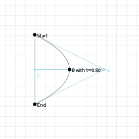
For cubic curves we need to do a little more work, but really only just a little. We're first going to assume that a decent curve through the three points should approximate a circular arc, which first requires knowing how to fit a circle to three points. You may remember (if you ever learned it!) that a line between two points on a circle is called a chord, and that one property of chords is that the line from the center of any chord, perpendicular to that chord, passes through the center of the circle.
That means that if we have three points on a circle, we have three (different) chords, and consequently, three (different) lines that go from those chords through the center of the circle: if we find two of those lines, then their intersection will be our circle's center, and the circle's radius will—by definition!—be the distance from the center to any of our three points:
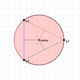
With that covered, we now also know the tangent line to our point B, because the tangent to any point on the circle is a line
through that point, perpendicular to the line from that point to the center. That just leaves marking appropriate points
e1 and e2 on that tangent, so that we can construct a new cubic curve hull. We use the approach as we did for
quadratic curves to automatically determine a reasonable t value, and then our e1 and
e2 coordinates must obey the standard de Casteljau rule for linear interpolation:

Where d is the total length of the line segment from e1 to e2. So how long do we make that? There
are again all kinds of approaches we can take, and a simple-but-effective one is to set the length of that segment to "one third the
length of the baseline". This forces e1 and e2 to always be the "linear curve" distance apart, which means if we
place our three points on a line, it will actually look like a line. Nice! The last thing we'll need to do is make sure to flip
the sign of d depending on which side of the baseline our B is located, so we don't end up creating a funky
curve with a loop in it. To do this, we can use the atan2 function:

This angle φ will be between 0 and π if B is "above" the baseline (rotating all three points so that the start is on the left
and the end is the right), so we can use a relatively straight forward check to make sure we're using the correct sign for our value
d:

The result of this approach looks as follows:
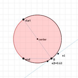
It is important to remember that even though we're using a circular arc to come up with decent e1 and e2 terms,
we're not trying to perfectly create a circular arc with a cubic curve (which is good, because we can't;
more on that later), we're only trying to come up with some reasonable e1 and
e2 points so we can construct a new cubic curve... so now that we have those: let's see what kind of cubic curve that gives
us:
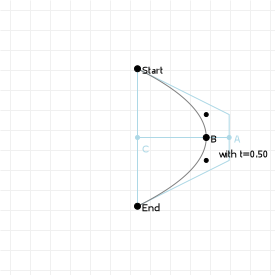
That looks perfectly serviceable!
Of course, we can take this one step further: we can't just "create" curves, we also have (almost!) all the tools available to "mold" curves, where we can reshape a curve by dragging a point on the curve around while leaving the start and end fixed, effectively molding the shape as if it were clay or the like. We'll see the last tool we need to do that in the next section, and then we'll look at implementing curve molding in the section after that, so read on!
Projecting a point onto a Bézier curve
Before we can move on to actual curve molding, it'll be good if know how to actually be able to find "some point on the curve" that we're trying to click on. After all, if all we have is our Bézier coordinates, that is not in itself enough to figure out which point on the curve our cursor will be closest to. So, how do we project points onto a curve?
If the Bézier curve is of low enough order, we might be able to
work out the maths for how to do this, and get a perfect t value back, but in general this is an incredibly hard problem and the easiest solution is, really, a
numerical approach again. We'll be finding our ideal t value using a
binary search. First, we do a coarse distance-check based on
t values associated with the curve's "to draw" coordinates (using a lookup table, or LUT). This is pretty fast:
| 1 | |
| 2 | |
| 3 | |
| 4 | |
| 5 | |
| 6 | |
| 7 | |
| 8 |
After this runs, we know that LUT[i] is the coordinate on the curve in our LUT that is closest to the point we want
to project, so that's a pretty good initial guess as to what the best projection onto our curve is. To refine it, we note that
LUT[i] is a better guess than both LUT[i-1] and LUT[i+1], but there might be an even better
projection somewhere else between those two values, so that's what we're going to be testing for, using a variation of the binary
search.
-
we start with our point
p, and thetvaluest1=LUT[i-1].tandt2=LUT[i+1].t, which span an intervalv = t2-t1. - we test this interval in five spots: the start, middle, and end (which we already have), and the two points in between the middle and start/end points
-
we then check which of these five points is the closest to our original point
p, and then repeat step 1 with the points before and after the closest point we just found.
This makes the interval we check smaller and smaller at each iteration, and we can keep running the three steps until the interval becomes so small as to lead to distances that are, for all intents and purposes, the same for all points.
So, let's see that in action: in this case, I'm going to arbitrarily say that if we're going to run the loop until the interval is smaller than 0.001, and show you what that means for projecting your mouse cursor or finger tip onto a rather complex Bézier curve (which, of course, you can reshape as you like). Also shown are the original three points that our coarse check finds.
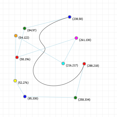
Intersections with a circle
It might seem odd to cover this subject so much later than the line/line, line/curve, and curve/curve intersection topics from several sections earlier, but the reason we can't cover circle/curve intersections is that we can't really discuss circle/curve intersection until we've covered the kind of lookup table (LUT) walking that the section on projecting a point onto a curve uses. To see why, let's look at what we would have to do if we wanted to find the intersections between a curve and a circle using calculus.
First, we observe that "finding intersections" in this case means that, given a circle defined by a center point
c = (x,y) and a radius r, we want to find all points on the Bezier curve for which the distance to the circle's
center point is equal to the circle radius, which by definition means those points lie on the circle, and so count as intersections. In
maths, that means we're trying to solve:

Which seems simple enough. Unfortunately, when we expand that dist function, things get a lot more problematic:

And now we have a problem because that's a sixth degree polynomial inside the square root. So, thanks to the Abel-Ruffini theorem that we saw before, we can't solve this by just going "square both sides because we don't care about signs"... we can't solve a sixth degree polynomial. So, we're going to have to actually evaluate that expression. We can "simplify" this by translating all our coordinates so that the center of the circle is (0,0) and all our coordinates are shifted accordingly, which makes the cx and cy terms fall away, but then we're still left with a monstrous function to solve.
So instead, we turn to the same kind of "LUT walking" that we saw for projecting points onto a curve, with a twist: instead of finding the
on-curve point with the smallest distance to our projection point, we want to find the on-curve point that has the exact distance
r to our projection point (namely, our circle center). Of course, there can be more than one such point, so there's also a
bit more code to make sure we find all of them, but let's look at the steps involved:
| 1 | |
| 2 | |
| 3 | |
| 4 | |
| 5 | |
| 6 | |
| 7 | |
| 8 | |
| 9 |
This is very similar to the code in the previous section, with an extra input r for the circle radius, and a minor
change in the "distance for this coordinate": rather than just distance(coordinate, p) we want to know the difference between
that distance and the circle radius. After all, if that difference is zero, then the distance from the coordinate to the circle center is
exactly the radius, so the coordinate lies on both the curve and the circle.
So far so good.
However, we also want to make sure we find all the points, not just a single one, so we need a little more code for that:
| 1 | |
| 2 | |
| 3 | |
| 4 | |
| 5 | |
| 6 | |
| 7 | |
| 8 | |
| 9 | |
| 10 |
After running this code, values will be the list of all LUT coordinates that are closest to the distance r: we
can use those values to run the same kind of refinement lookup we used for point projection (with the caveat that we're now
not checking for smallest distance, but for "distance closest to r"), and we'll have all our intersection points. Of
course, that does require explaining what findClosest does: rather than looking for a global minimum, we're now interested in
finding a local minimum, so instead of checking a single point and looking at its distance value, we check three points
("current", "previous" and "before previous") and then check whether they form a local minimum:
| 1 | |
| 2 | |
| 3 | |
| 4 | |
| 5 | |
| 6 | |
| 7 | |
| 8 | |
| 9 | |
| 10 | |
| 11 | |
| 12 | |
| 13 | |
| 14 | |
| 15 | |
| 16 | |
| 17 | |
| 18 | |
| 19 |
In words: given a start index, the circle center and radius, and our LUT, we check where (closest to our
start index) we can find a local minimum for the difference between "the distance from the curve to the circle center", and
the circle's radius. We track this by looking at three values (associated with the indices index-2, index-1, and
index), and we know we've found a local minimum if the three values show that the middle value (pd1) is less
than either value beside it. When we do, we can set our "best guess, relative to start" as index-1. Of course,
since we're now checking values relative to some start value, we might not find another candidate value at all, in which case
we return start - 1, so that a simple "is the result less than start?" lets us determine that there are no more
intersections to find.
Finally, while not necessary for point projection, there is one more step we need to perform when we run the binary refinement function on
our candidate LUT indices, because we've so far only been testing using distances "closest to the radius of the circle", and that's
actually not good enough... we need distances that are the radius of the circle. So, after running the refinement for each of
these indices, we need to discard any final value that isn't the circle radius. And because we're working with floating point numbers,
what this really means is that we need to discard any value that's a pixel or more "off". Or, if we want to get really fancy, "some small
epsilon value".
Based on all of that, the following graphic shows this off for the standard cubic curve (which you can move the coordinates around for, of course) and a circle with a controllable radius centered on the graphic's center, using the code approach described above.
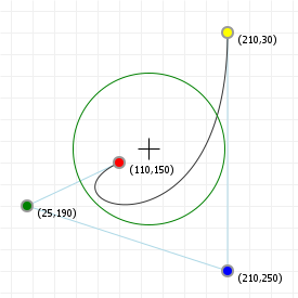
And of course, for the full details, click that "view source" link.
Molding a curve
Armed with knowledge of the "ABC" relation, point-on-curve projection, and guestimating reasonable looking helper values for cubic curve construction, we can finally cover curve molding: updating a curve's shape interactively, by dragging points on the curve around.
For quadratic curve, this is a really simple trick: we project our cursor onto the curve, which gives us a t value and
initial B coordinate. We don't even need the latter: with our t value and "wherever the cursor is" as target
B, we can compute the associated C:

And then the associated A:

And we're done, because that's our new quadratic control point!
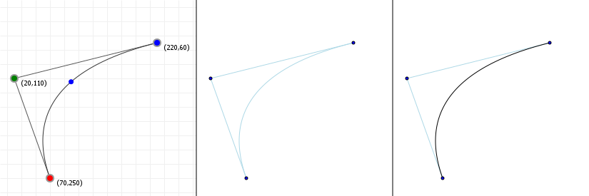
As before, cubic curves are a bit more work, because while it's easy to find our initial t value and ABC values, getting
those all-important e1 and e2 coordinates is going to pose a bit of a problem... in the section on curve
creation, we were free to pick an appropriate t value ourselves, which allowed us to find appropriate e1 and
e2 coordinates. That's great, but when we're curve molding we don't have that luxury: whatever point we decide to start
moving around already has its own t value, and its own e1 and e2 values, and those may not make
sense for the rest of the curve.
For example, let's see what happens if we just "go with what we get" when we pick a point and start moving it around, preserving its
t value and e1/e2 coordinates:
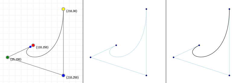
That looks reasonable, close to the original point, but the further we drag our point, the less "useful" things become. Especially if we drag our point across the baseline, rather than turning into a nice curve.
One way to combat this might be to combine the above approach with the approach from the
creating curves section: generate both the "unchanged t/e1/e2" curve, as
well as the "idealized" curve through the start/cursor/end points, with idealized t value, and then interpolating between
those two curves:

The slide controls the "falloff distance" relative to where the original point on the curve is, so that as we drag our point around, it
interpolates with a bias towards "preserving t/e1/e2" closer to the original point, and bias
towards "idealized" form the further away we move our point, with anything that's further than our falloff distance simply
being the idealized curve. We don't even try to interpolate at that point.
A more advanced way to try to smooth things out is to implement continuous molding, where we constantly update the curve as we
move around, and constantly change what our B point is, based on constantly projecting the cursor on the curve
as we're updating it - this is, you won't be surprised to learn, tricky, and beyond the scope of this section: interpolation
(with a reasonable distance) will do for now!
Curve fitting
Given the previous section, one question you might have is "what if I don't want to guess t values?". After all, plenty of
graphics packages do automated curve fitting, so how can we implement that in a way that just finds us reasonable t values
all on its own?
And really this is just a variation on the question "how do I get the curve through these X points?", so let's look at that. Specifically,
let's look at the answer: "curve fitting". This is in fact a rather rich field in geometry, applying to anything from data modelling to
path abstraction to "drawing", so there's a fair number of ways to do curve fitting, but we'll look at one of the most common approaches:
something called a least squares
polynomial regression. In this approach, we look at the number of points
we have in our data set, roughly determine what would be an appropriate order for a curve that would fit these points, and then tackle the
question "given that we want an nth order curve, what are the coordinates we can find such that our curve is "off" by the
least amount?".
Now, there are many ways to determine how "off" points are from the curve, which is where that "least squares" term comes in. The most common tool in the toolbox is to minimise the squared distance between each point we have, and the corresponding point on the curve we end up "inventing". A curve with a snug fit will have zero distance between those two, and a bad fit will have non-zero distances between every such pair. It's a workable metric. You might wonder why we'd need to square, rather than just ensure that distance is a positive value (so that the total error is easy to compute by just summing distances) and the answer really is "because it tends to be a little better". There's lots of literature on the web if you want to deep-dive the specific merits of least squared error metrics versus least absolute error metrics, but those are well beyond the scope of this material.
So let's look at what we end up with in terms of curve fitting if we start with the idea of performing least squares Bézier fitting. We're going to follow a procedure similar to the one described by Jim Herold over on his "Least Squares Bézier Fit" article, and end with some nice interactive graphics for doing some curve fitting.
Before we begin, we're going to use the curve in matrix form. In the section on matrices, I mentioned that some things are easier if we use the matrix representation of a Bézier curve rather than its calculus form, and this is one of those things.
As such, the first step in the process is expressing our Bézier curve as powers/coefficients/coordinate matrix T x M x C, by expanding the Bézier functions.
Revisiting the matrix representation
Rewriting Bézier functions to matrix form is fairly easy, if you first expand the function, and then arrange them into a multiple line form, where each line corresponds to a power of t, and each column is for a specific coefficient. First, we expand the function:

And then we (trivially) rearrange the terms across multiple lines:

This rearrangement has "factors of t" at each row (the first row is t⁰, i.e. "1", the second row is t¹, i.e. "t", the third row is t²) and "coefficient" at each column (the first column is all terms involving "a", the second all terms involving "b", the third all terms involving "c").
With that arrangement, we can easily decompose this as a matrix multiplication:

We can do the same for the cubic curve, of course. We know the base function for cubics:

So we write out the expansion and rearrange:

Which we can then decompose:

And, of course, we can do this for quartic curves too (skipping the expansion step):

And so and on so on. Now, let's see how to use these T, M, and C, to do some curve fitting.
Let's get started: we're going to assume we picked the right order curve: for n points we're fitting an n-1th order curve, so we "start" with a vector P that represents the coordinates we already know, and for which
we want to do curve fitting:

Next, we need to figure out appropriate t values for each point in the curve, because we need something that lets us tie "the
actual coordinate" to "some point on the curve". There's a fair number of different ways to do this (and a large part of optimizing "the
perfect fit" is about picking appropriate t values), but in this case let's look at two "obvious" choices:
- equally spaced
tvalues, and tvalues that align with distance along the polygon.
The first one is really simple: if we have n points, then we'll just assign each point i a t value
of (i-1)/(n-1). So if we have four points, the first point will have t=(1-1)/(4-1)=0/3, the second point will
have t=(2-1)/(4-1)=1/3, the third point will have t=2/3, and the last point will be t=1. We're just
straight up spacing the t values to match the number of points we have.
The second one is a little more interesting: since we're doing polynomial regression, we might as well exploit the fact that our base
coordinates just constitute a collection of line segments. At the first point, we're fixing t=0, and the last point, we want t=1, and
anywhere in between we're simply going to say that t is equal to the distance along the polygon, scaled to the [0,1] domain.
To get these values, we first compute the general "distance along the polygon" matrix:

Where length() is literally just that: the length of the line segment between the point we're looking at, and the previous
point. This isn't quite enough, of course: we still need to make sure that all the values between i=1 and
i=n fall in the [0,1] interval, so we need to scale all values down by whatever the total length of the polygon is:

And now we can move on to the actual "curve fitting" part: what we want is a function that lets us compute "ideal" control point values such that if we build a Bézier curve with them, that curve passes through all our original points. Or, failing that, have an overall error distance that is as close to zero as we can get it. So, let's write out what the error distance looks like.
As mentioned before, this function is really just "the distance between the actual coordinate, and the coordinate that the curve evaluates
to for the associated t value", which we'll square to get rid of any pesky negative signs:

Since this function only deals with individual coordinates, we'll need to sum over all coordinates in order to get the full error function. So, we literally just do that; the total error function is simply the sum of all these individual errors:

And here's the trick that justifies using matrices: while we can work with individual values using calculus, with matrices we can compute as many values as we make our matrices big, all at the "same time", We can replace the individual terms pi with the full P coordinate matrix, and we can replace Bézier(si) with the matrix representation T x M x C we talked about before, which gives us:

In which we can replace the rather cumbersome "squaring" operation with a more conventional matrix equivalent:

Here, the letter T is used instead of the number 2, to represent the
matrix transpose; each row in the original matrix becomes a column in the transposed
matrix instead (row one becomes column one, row two becomes column two, and so on).
This leaves one problem: T isn't actually the matrix we want: we don't want symbolic t values, we want the
actual numerical values that we computed for S, so we need to form a new matrix, which we'll call 𝕋, that makes use of
those, and then use that 𝕋 instead of T in our error function:

Which, because of the first and last values in S, means:

Now we can properly write out the error function as matrix operations:

So, we have our error function: we now need to figure out the expression for where that function has minimal value, e.g. where the error between the true coordinates and the coordinates generated by the curve fitting is smallest. Like in standard calculus, this requires taking the derivative, and determining where that derivative is zero:

Where did this derivative come from?
That... is a good question. In fact, when trying to run through this approach, I ran into the same question! And you know what? I straight up had no idea. I'm decent enough at calculus, I'm decent enough at linear algebra, and I just don't know.
So I did what I always do when I don't understand something: I asked someone to help me understand how things work. In this specific case, I posted a question to Math.stackexchange, and received a answer that goes into way more detail than I had hoped to receive.
Is that answer useful to you? Probably: no. At least, not unless you like understanding maths on a recreational level. And I do mean maths in general, not just basic algebra. But it does help in giving us a reference in case you ever wonder "Hang on. Why was that true?". There are answers. They might just require some time to come to understand.
Now, given the above derivative, we can rearrange the terms (following the rules of matrix algebra) so that we end up with an expression for C:

Here, the "to the power negative one" is the notation for the
matrix inverse. But that's all we have to do: we're done. Starting with
P and inventing some t values based on the polygon the coordinates in P define, we can
compute the corresponding Bézier coordinates C that specify a curve that goes through our points. Or, if it can't go
through them exactly, as near as possible.
So before we try that out, how much code is involved in implementing this? Honestly, that answer depends on how much you're going to be writing yourself. If you already have a matrix maths library available, then really not that much code at all. On the other hand, if you are writing this from scratch, you're going to have to write some utility functions for doing your matrix work for you, so it's really anywhere from 50 lines of code to maybe 200 lines of code. Not a bad price to pay for being able to fit curves to pre-specified coordinates.
So let's try it out! The following graphic lets you place points, and will start computing exact-fit curves once you've placed at least three. You can click for more points, and the code will simply try to compute an exact fit using a Bézier curve of the appropriate order. Four points? Cubic Bézier. Five points? Quartic. And so on. Of course, this does break down at some point: depending on where you place your points, it might become mighty hard for the fitter to find an exact fit, and things might actually start looking horribly off once there's enough points for compound floating point rounding errors to start making a difference (which is around 10~11 points).
You'll note there is a convenient "toggle" buttons that lets you toggle between equidistant t values, and distance ratio
along the polygon formed by the points. Arguably more interesting is that once you have points to abstract a curve, you also get
direct control over the time values through sliders for each, because if the time values are our degree of freedom, you should be
able to freely manipulate them and see what the effect on your curve is.
Bézier curves and Catmull-Rom curves
Taking an excursion to different splines, the other common design curve is the Catmull-Rom spline, which unlike Bézier curves pass through each control point, so they offer a kind of "built-in" curve fitting.
In fact, let's start with just playing with one: the following graphic has a predefined curve that you manipulate the points for, and lets you add points by clicking/tapping the background, as well as let you control "how fast" the curve passes through its point using the tension slider. The tenser the curve, the more the curve tends towards straight lines from one point to the next.
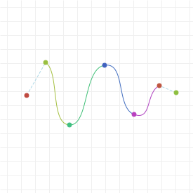
Now, it may look like Catmull-Rom curves are very different from Bézier curves, because these curves can get very long indeed, but what looks like a single Catmull-Rom curve is actually a spline: a single curve built up of lots of identically-computed pieces, similar to if you just took a whole bunch of Bézier curves, placed them end to end, and lined up their control points so that things look like a single curve. For a Catmull-Rom curve, each "piece" between two points is defined by the point's coordinates, and the tangent for those points, the latter of which can trivially be derived from knowing the previous and next point:

One downside of this is that—as you may have noticed from the graphic—the first and last point of the overall curve don't actually join up with the rest of the curve: they don't have a previous/next point respectively, and so there is no way to calculate what their tangent should be. Which also makes it rather tricky to fit a Catmull-Rom curve to three points like we were able to do for Bézier curves. More on that in the next section.
In fact, before we move on, let's look at how to actually draw the basic form of these curves (I say basic, because there are a number of variations that make things considerable more complex):
| 1 | |
| 2 | |
| 3 | |
| 4 | |
| 5 | |
| 6 | |
| 7 | |
| 8 | |
| 9 | |
| 10 | |
| 11 | |
| 12 | |
| 13 | |
| 14 | |
| 15 | |
| 16 | |
| 17 | |
| 18 | |
| 19 |
Now, since a Catmull-Rom curve is a form of cubic Hermite spline, and as cubic Bézier curves are also a form of cubic Hermite spline, we run into an interesting bit of maths programming: we can convert one to the other and back, and the maths for doing so is surprisingly simple!
The main difference between Catmull-Rom curves and Bézier curves is "what the points mean":
- A cubic Bézier curve is defined by a start point, a control point that implies the tangent at the start, a control point that implies the tangent at the end, and an end point, plus a characterizing matrix that we can multiply by that point vector to get on-curve coordinates.
- A Catmull-Rom curve is defined by a start point, a tangent that for that starting point, an end point, and a tangent for that end point, plus a characteristic matrix that we can multiple by the point vector to get on-curve coordinates.
Those are very similar, so let's see exactly how similar they are. We've already see the matrix form for Bézier curves, so how different is the matrix form for Catmull-Rom curves?:

That's pretty dang similar. So the question is: how can we convert that expression with Catmull-Rom matrix and vector into an expression of the Bézier matrix and vector? The short answer is of course "by using linear algebra", but the longer answer is the rest of this section, and involves some maths that you may not even care for: if you just want to know the (incredibly simple) conversions between the two curve forms, feel free to skip to the end of the following explanation, but if you want to how we can get one from the other... let's get mathing!
Deriving the conversion formulae
In order to convert between Catmull-Rom curves and Bézier curves, we need to know two things. Firstly, how to express the Catmull-Rom curve using a "set of four coordinates", rather than a mix of coordinates and tangents, and secondly, how to convert those Catmull-Rom coordinates to and from Bézier form.
We start with the first part, to figure out how we can go from Catmull-Rom V coordinates to Bézier P coordinates, by applying "some matrix T". We don't know what that T is yet, but we'll get to that:

So, this mapping says that in order to map a Catmull-Rom "point + tangent" vector to something based on an "all coordinates" vector, we need to determine the mapping matrix such that applying T yields P2 as start point, P3 as end point, and two tangents based on the lines between P1 and P3, and P2 nd P4, respectively.
Computing T is really more "arranging the numbers":

Thus:

However, we're not quite done, because Catmull-Rom curves have that "tension" parameter, written as τ (a lowercase"tau"), which is a scaling factor for the tangent vectors: the bigger the tension, the smaller the tangents, and the smaller the tension, the bigger the tangents. As such, the tension factor goes in the denominator for the tangents, and before we continue, let's add that tension factor into both our coordinate vector representation, and mapping matrix T:

With the mapping matrix properly done, let's rewrite the "point + tangent" Catmull-Rom matrix form to a matrix form in terms of four coordinates, and see what we end up with:

Replace point/tangent vector with the expression for all-coordinates:

and merge the matrices:

This looks a lot like the Bézier matrix form, which as we saw in the chapter on Bézier curves, should look like this:

So, if we want to express a Catmull-Rom curve using a Bézier curve, we'll need to turn this Catmull-Rom bit:

Into something that looks like this:

And the way we do that is with a fairly straight forward bit of matrix rewriting. We start with the equality we need to ensure:

Then we remove the coordinate vector from both sides without affecting the equality:

Then we can "get rid of" the Bézier matrix on the right by left-multiply both with the inverse of the Bézier matrix:

A matrix times its inverse is the matrix equivalent of 1, and because "something times 1" is the same as "something", so we can just outright remove any matrix/inverse pair:

And now we're basically done. We just multiply those two matrices and we know what V is:

We now have the final piece of our function puzzle. Let's run through each step.
- Start with the Catmull-Rom function:

- rewrite to pure coordinate form:

- rewrite for "normal" coordinate vector:

- merge the inner matrices:

- rewrite for Bézier matrix form:

- and transform the coordinates so we have a "pure" Bézier expression:

And we're done: we finally know how to convert these two curves!
If we have a Catmull-Rom curve defined by four coordinates P1 through P4, then we can draw that curve using a Bézier curve that has the vector:

Similarly, if we have a Bézier curve defined by four coordinates P1 through P4, we can draw that using a standard tension Catmull-Rom curve with the following coordinate values:

Or, if your API allows you to specify Catmull-Rom curves using plain coordinates:

Creating a Catmull-Rom curve from three points
Much shorter than the previous section: we saw that Catmull-Rom curves need at least 4 points to draw anything sensible, so how do we create a Catmull-Rom curve from three points?
Short and sweet: we don't.
We run through the maths that lets us create a cubic Bézier curve, and then convert its coordinates to Catmull-Rom form using the conversion formulae we saw above.
Forming poly-Bézier curves
Much like lines can be chained together to form polygons, Bézier curves can be chained together to form poly-Béziers, and the only trick required is to make sure that:
- the end point of each section is the starting point of the following section, and
- the derivatives across that dual point line up.
Unless you want sharp corners, of course. Then you don't even need 2.
We'll cover three forms of poly-Bézier curves in this section. First, we'll look at the kind that just follows point 1. where the end point of a segment is the same point as the start point of the next segment. This leads to poly-Béziers that are pretty hard to work with, but they're the easiest to implement:

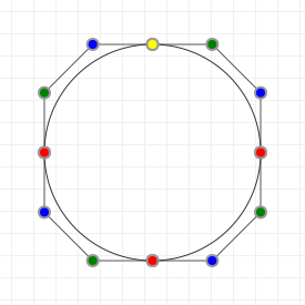
Dragging the control points around only affects the curve segments that the control point belongs to, and moving an on-curve point leaves the control points where they are, which is not the most useful for practical modelling purposes. So, let's add in the logic we need to make things a little better. We'll start by linking up control points by ensuring that the "incoming" derivative at an on-curve point is the same as it's "outgoing" derivative:

We can effect this quite easily, because we know that the vector from a curve's last control point to its last on-curve point is equal to the derivative vector. If we want to ensure that the first control point of the next curve matches that, all we have to do is mirror that last control point through the last on-curve point. And mirroring any point A through any point B is really simple:

So let's implement that and see what it gets us. The following two graphics show a quadratic and a cubic poly-Bézier curve again, but this time moving the control points around moves others, too. However, you might see something unexpected going on for quadratic curves...


As you can see, quadratic curves are particularly ill-suited for poly-Bézier curves, as all the control points are effectively linked. Move one of them, and you move all of them. Not only that, but if we move the on-curve points, it's possible to get a situation where a control point cannot satisfy the constraint that it's the reflection of its two neighbouring control points... This means that we cannot use quadratic poly-Béziers for anything other than really, really simple shapes. And even then, they're probably the wrong choice. Cubic curves are pretty decent, but the fact that the derivatives are linked means we can't manipulate curves as well as we might if we relaxed the constraints a little.
So: let's relax the requirement a little.
We can change the constraint so that we still preserve the angle of the derivatives across sections (so transitions from one section to the next will still look natural), but give up the requirement that they should also have the same vector length. Doing so will give us a much more useful kind of poly-Bézier curve:


Cubic curves are now better behaved when it comes to dragging control points around, but the quadratic poly-Bézier still has the problem that moving one control points will move the control points and may ending up defining "the next" control point in a way that doesn't work. Quadratic curves really aren't very useful to work with...
Finally, we also want to make sure that moving the on-curve coordinates preserves the relative positions of the associated control points. With that, we get to the kind of curve control that you might be familiar with from applications like Photoshop, Inkscape, Blender, etc.
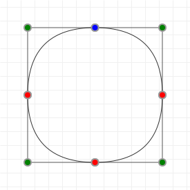

Again, we see that cubic curves are now rather nice to work with, but quadratic curves have a new, very serious problem: we can move an on-curve point in such a way that we can't compute what needs to "happen next". Move the top point down, below the left and right points, for instance. There is no way to preserve correct control points without a kink at the bottom point. Quadratic curves: just not that good...
A final improvement is to offer fine-level control over which points behave which, so that you can have "kinks" or individually controlled segments when you need them, with nicely well-behaved curves for the rest of the path. Implementing that, is left as an exercise for the reader.
Curve offsetting
Perhaps you're like me, and you've been writing various small programs that use Bézier curves in some way or another, and at some point you make the step to implementing path extrusion. But you don't want to do it pixel based; you want to stay in the vector world. You find that extruding lines is relatively easy, and tracing outlines is coming along nicely (although junction caps and fillets are a bit of a hassle), and then you decide to do things properly and add Bézier curves to the mix. Now you have a problem.
Unlike lines, you can't simply extrude a Bézier curve by taking a copy and moving it around, because of the curvatures; rather than a uniform thickness, you get an extrusion that looks too thin in places, if you're lucky, but more likely will self-intersect. The trick, then, is to scale the curve, rather than simply copying it. But how do you scale a Bézier curve?
Bottom line: you can't. So you cheat. We're not going to do true curve scaling, or rather curve offsetting, because that's impossible. Instead we're going to try to generate 'looks good enough' offset curves.
"What do you mean, you can't? Prove it."
First off, when I say "you can't," what I really mean is "you can't offset a Bézier curve with another Bézier curve", not even by using a really high order curve. You can find the function that describes the offset curve, but it won't be a polynomial, and as such it cannot be represented as a Bézier curve, which has to be a polynomial. Let's look at why this is:
From a mathematical point of view, an offset curve O(t) is a curve such that, given our original curve B(t),
any point on O(t) is a fixed distance d away from coordinate B(t). So let's math that:

However, we're working in 2D, and d is a single value, so we want to turn it into a vector. If we want a point distance
d "away" from the curve B(t) then what we really mean is that we want a point at d times the
"normal vector" from point B(t), where the "normal" is a vector that runs perpendicular ("at a right angle") to the tangent
at B(t). Easy enough:

Now this still isn't very useful unless we know what the formula for N(t) is, so let's find out. N(t) runs
perpendicular to the original curve tangent, and we know that the tangent is simply B'(t), so we could just rotate that 90
degrees and be done with it. However, we need to ensure that N(t) has the same magnitude for every t, or the
offset curve won't be at a uniform distance, thus not being an offset curve at all. The easiest way to guarantee this is to make sure
N(t) always has length 1, which we can achieve by dividing B'(t) by its magnitude:

The magnitude of B'(t), usually denoted with double vertical bars, is given by the following formula:

And that's where things go wrong: that square root is screwing everything up, because it turns our nice polynomials into things that are no longer polynomials.
There is a small class of polynomials where the square root is also a polynomial, but they're utterly useless to us: any polynomial with unweighted binomial coefficients has a square root that is also a polynomial. Now, you might think that Bézier curves are just fine because they do, but they don't; remember that only the base function has binomial coefficients. That's before we factor in our coordinates, which turn it into a non-binomial polygon. The only way to make sure the functions stay binomial is to make all our coordinates have the same value. And that's not a curve, that's a point. We can already create offset curves for points, we call them circles, and they have much simpler functions than Bézier curves.
So, since the tangent length isn't a polynomial, the normalised tangent won't be a polynomial either, which means
N(t) won't be a polynomial, which means that d times N(t) won't be a polynomial, which means
that, ultimately, O(t) won't be a polynomial, which means that even if we can determine the function for
O(t) just fine (and that's far from trivial!), it simply cannot be represented as a Bézier curve.
And that's one reason why Bézier curves are tricky: there are actually a lot of curves that cannot be represented as a Bézier curve at all. They can't even model their own offset curves. They're weird that way. So how do all those other programs do it? Well, much like we're about to do, they cheat. We're going to approximate an offset curve in a way that will look relatively close to what the real offset curve would look like, if we could compute it.
So, you cannot offset a Bézier curve perfectly with another Bézier curve, no matter how high-order you make that other Bézier curve.
However, we can chop up a curve into "safe" sub-curves (where "safe" means that all the control points are always on a single side of the
baseline, and the midpoint of the curve at t=0.5 is roughly in the center of the polygon defined by the curve coordinates)
and then point-scale each sub-curve with respect to its scaling origin (which is the intersection of the point normals at the start and
end points).
A good way to do this reduction is to first find the curve's extreme points, as explained in the earlier section on curve extremities, and
use these as initial splitting points. After this initial split, we can check each individual segment to see if it's "safe enough" based
on where the center of the curve is. If the on-curve point for t=0.5 is too far off from the center, we simply split the
segment down the middle. Generally this is more than enough to end up with safe segments.
The following graphics show off curve offsetting, and you can use the slider to control the distance at which the curve gets offset. The curve first gets reduced to safe segments, each of which is then offset at the desired distance. Especially for simple curves, particularly easily set up for quadratic curves, no reduction is necessary, but the more twisty the curve gets, the more the curve needs to be reduced in order to get segments that can safely be scaled.
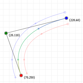
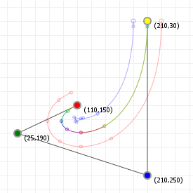
You may notice that this may still lead to small 'jumps' in the sub-curves when moving the curve around. This is caused by the fact that we're still performing a naive form of offsetting, moving the control points the same distance as the start and end points. If the curve is large enough, this may still lead to incorrect offsets.
Graduated curve offsetting
What if we want to do graduated offsetting, starting at some distance s but ending at some other distance e?
Well, if we can compute the length of a curve (which we can if we use the Legendre-Gauss quadrature approach) then we can also determine
how far "along the line" any point on the curve is. With that knowledge, we can offset a curve so that its offset curve is not uniformly
wide, but graduated between with two different offset widths at the start and end.
Like normal offsetting we cut up our curve in sub-curves, and then check at which distance along the original curve each sub-curve starts
and ends, as well as to which point on the curve each of the control points map. This gives us the distance-along-the-curve for each
interesting point in the sub-curve. If we call the total length of all sub-curves seen prior to seeing "the current" sub-curve
S (and if the current sub-curve is the first one, S is zero), and we call the full length of our original curve
L, then we get the following graduation values:
- start: map
Sfrom interval (0,L) to interval(s,e) - c1:
map(<strong>S+d1</strong>, 0,L, s,e), d1 = distance along curve to projection of c1 - c2:
map(<strong>S+d2</strong>, 0,L, s,e), d2 = distance along curve to projection of c2 - ...
- end:
map(<strong>S+length(subcurve)</strong>, 0,L, s,e)
At each of the relevant points (start, end, and the projections of the control points onto the curve) we know the curve's normal, so offsetting is simply a matter of taking our original point, and moving it along the normal vector by the offset distance for each point. Doing so will give us the following result (these have with a starting width of 0, and an end width of 40 pixels, but can be controlled with your up and down arrow keys):
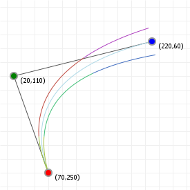
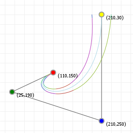
Circles and quadratic Bézier curves
Circles and Bézier curves are very different beasts, and circles are infinitely easier to work with than Bézier curves. Their formula is much simpler, and they can be drawn more efficiently. But, sometimes you don't have the luxury of using circles, or ellipses, or arcs. Sometimes, all you have are Bézier curves. For instance, if you're doing font design, fonts have no concept of geometric shapes, they only know straight lines, and Bézier curves. OpenType fonts with TrueType outlines only know quadratic Bézier curves, and OpenType fonts with Type 2 outlines only know cubic Bézier curves. So how do you draw a circle, or an ellipse, or an arc?
You approximate.
We already know that Bézier curves cannot model all curves that we can think of, and this includes perfect circles, as well as ellipses, and their arc counterparts. However, we can certainly approximate them to a degree that is visually acceptable. Quadratic and cubic curves offer us different curvature control, so in order to approximate a circle we will first need to figure out what the error is if we try to approximate arcs of increasing degree with quadratic and cubic curves, and where the coordinates even lie.
Since arcs are mid-point-symmetrical, we need the control points to set up a symmetrical curve. For quadratic curves this means that the control point will be somewhere on a line that intersects the baseline at a right angle. And we don't get any choice on where that will be, since the derivatives at the start and end point have to line up, so our control point will lie at the intersection of the tangents at the start and end point.
First, let's try to fit the quadratic curve onto a circular arc. In the following sketch you can move the mouse around over a unit circle, to see how well, or poorly, a quadratic curve can approximate the arc from (1,0) to where your mouse cursor is:
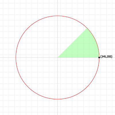
As you can see, things go horribly wrong quite quickly; even trying to approximate a quarter circle using a quadratic curve is a bad idea. An eighth of a turns might look okay, but how okay is okay? Let's apply some maths and find out. What we're interested in is how far off our on-curve coordinates are with respect to a circular arc, given a specific start and end angle. We'll be looking at how much space there is between the circular arc, and the quadratic curve's midpoint.
We start out with our start and end point, and for convenience we will place them on a unit circle (a circle around 0,0 with radius 1), at some angle φ:

What we want to find is the intersection of the tangents, so we want a point C such that:

i.e. we want a point that lies on the vertical line through S (at some distance a from S) and also lies on the tangent line through E (at some distance b from E). Solving this gives us:

First we solve for b:

which yields:

which we can then substitute in the expression for a:

A quick check shows that plugging these values for a and b into the expressions for Cx and Cy give the same x/y coordinates for both "a away from A" and "b away from B", so let's continue: now that we know the coordinate values for C, we know where our on-curve point T for t=0.5 (or angle φ/2) is, because we can just evaluate the Bézier polynomial, and we know where the circle arc's actual point P is for angle φ/2:

We compute T, observing that if t=0.5, the polynomial values (1-t)², 2(1-t)t, and t² are 0.25, 0.5, and 0.25 respectively:

Which, worked out for the x and y components, gives:

And the distance between these two is the standard Euclidean distance:

So, what does this distance function look like when we plot it for a number of ranges for the angle φ, such as a half circle, quarter circle and eighth circle?
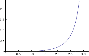 plotted for 0 ≤ φ ≤ π:
|
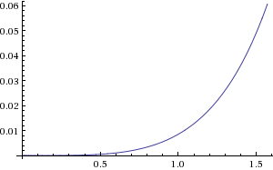 plotted for 0 ≤ φ ≤ ½π:
|
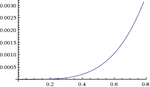 plotted for 0 ≤ φ ≤ ¼π:
|
We now see why the eighth circle arc looks decent, but the quarter circle arc doesn't: an error of roughly 0.06 at t=0.5 means we're 6% off the mark... we will already be off by one pixel on a circle with pixel radius 17. Any decent sized quarter circle arc, say with radius 100px, will be way off if approximated by a quadratic curve! For the eighth circle arc, however, the error is only roughly 0.003, or 0.3%, which explains why it looks so close to the actual eighth circle arc. In fact, if we want a truly tiny error, like 0.001, we'll have to contend with an angle of (rounded) 0.593667, which equates to roughly 34 degrees. We'd need 11 quadratic curves to form a full circle with that precision! (technically, 10 and ten seventeenth, but we can't do partial curves, so we have to round up). That's a whole lot of curves just to get a shape that can be drawn using a simple function!
In fact, let's flip the function around, so that if we plug in the precision error, labelled ε, we get back the maximum angle for that precision:

And frankly, things are starting to look a bit ridiculous at this point, we're doing way more maths than we've ever done, but thankfully this is as far as we need the maths to take us: If we plug in the precisions 0.1, 0.01, 0.001 and 0.0001 we get the radians values 1.748, 1.038, 0.594 and 0.3356; in degrees, that means we can cover roughly 100 degrees (requiring four curves), 59.5 degrees (requiring six curves), 34 degrees (requiring 11 curves), and 19.2 degrees (requiring a whopping nineteen curves).
The bottom line? Quadratic curves are kind of lousy if you want circular (or elliptical, which are circles that have been squashed in one dimension) curves. We can do better, even if it's just by raising the order of our curve once. So let's try the same thing for cubic curves.
Circular arcs and cubic Béziers
Let's look at approximating circles and circular arcs using cubic Béziers. How much better is that?
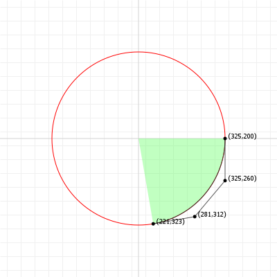
At cursory glance, a fair bit better, but let's find out how much better by looking at how to construct the Bézier curve.
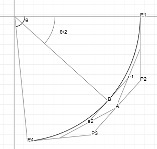
The start and end points are trivial, but the mid point requires a bit of work, but it's mostly basic trigonometry once we know the angle θ for our circular arc: if we scale our circular arc to a unit circle, we can always start our arc, with radius 1, at (1,0) and then given our arc angle θ, we also know that the circular arc has length θ (because unit circles are nice that way). We also know our end point, because that's just (cos(θ), sin(θ)), and so the challenge is to figure out what control points we need in order for the curve at t=0.5 to exactly touch the circular arc at the angle θ/2:
So let's again formally describe this:

Only P3 isn't quite straight-forward here, and its description is based on the fact that the triangle (origin, P4, P3) is a right angled triangle, with the distance between the origin and P4 being 1 (because we're working with a unit circle), and the distance between P4 and P3 being k, so that we can represent P3 as "The point P4 plus the vector from the origin to P4 but then rotated a quarter circle, counter-clockwise, and scaled by k".
With that, we can determine the y-coordinates for A, B, e1, and e2, after which we have all the information we need to determine what the value of k is. We can find these values by using (no surprise here) linear interpolation between known points, as A is midway between P2 and P3, e1 is between A and "midway between P1 and P2" (which is "half height" P2), and so forth:

Which now gives us two identities for B, because in addition to determining B through linear interpolation, we also know that B's y coordinate is just sin(θ/2): we started this exercise by saying we were going to approximate the circular arc using a Bézier curve that had its midpoint, which is point B, touching the unit circle at the arc's half-angle, by definition making B the point at (cos(θ/2), sin(θ/2)).
This means we can equate the two identities we now have for By and solve for k.
Deriving k
Solving for k is fairly straight forward, but it's a fair few steps, and if you just the immediate result: using a tool like Wolfram Alpha is definitely the way to go. That said, let's get going:

And finally, we can take further advantage of several trigonometric identities to drastically simplify our formula for k:

And we're done.
So, the distance of our control points to the start/end points can be expressed as a number that we get from an almost trivial expression involving the circular arc's angle:

Which means that for any circular arc with angle θ and radius r, our Bézier approximation based on three points of incidence is:

Which also gives us the commonly found value of 0.55228 for quarter circles, based on them having an angle of half π:

And thus giving us the following Bézier coordinates for a quarter circle of radius r:

So, how accurate is this?
Unlike for the quadratic curve, we can't use t=0.5 as our reference point because by its very nature it's one of the three points that are actually guaranteed to be on the circular arc itself. Instead, we need a different t value that will give us the maximum deflection - there are two possible choices (as our curve is still strictly "overshoots" the circular arc, and it's symmetrical) but rather than trying to use calculus to find the perfect t value—which we could! the maths is perfectly reasonable as long as we get to use computers—we can also just perform a binary search for the biggest deflection and not bother with all this maths stuff.
So let's do that instead: we can run a maximum deflection check that just runs through t from 0 to 1 at some coarse interval, finds a t value that has "the highest deflection of the bunch", then reruns the same check with a much smaller interval around that t value, repeating as many times as necessary to get us an arbitrarily precise value of t:
| 1 | |
| 2 | |
| 3 | |
| 4 | |
| 5 | |
| 6 | |
| 7 | |
| 8 | |
| 9 | |
| 10 | |
| 11 | |
| 12 | |
| 13 |
Plus, how often do you get to write a function with that name?
Using this code, we find that our t values are approximately 0.211325 and 0.788675, so let's pick the lower of the two and see what the maximum deflection is across our domain of angles, with the original quadratic error show in green (rocketing off to infinity first, and then coming back down as we approach 2π)
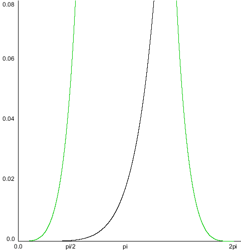
|
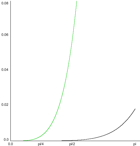
|
|
| error plotted for 0 ≤ φ ≤ 2π | error plotted for 0 ≤ φ ≤ π | error plotted for 0 ≤ φ ≤ ½π |
That last image is probably not quite clear enough: the cubic approximation of a quarter circle is so incredibly much better that we can't even really see it at the same scale of our quadratic curve. Let's scale the y-axis a little, and try that again:
Yeah... the error of a cubic approximation for a quarter circle turns out to be two orders of magnitude better. At approximately 0.00027 (or: just shy of being 2.7 pixels off for a circle with a radius of 10,000 pixels) the increase in precision over quadratic curves is quite spectacular - certainly good enough that no one in their right mind should ever use quadratic curves.
So that's it, kappa is 4/3 · tan(θ/4) , we're done! ...or are we?
Can we do better?
Technically: yes, we can. But I'm going to prefix this section with "we can, and we should investigate that possibility, but let me warn you up front that the result is only better if we're going to hard-code the values". We're about to get into the weeds and the standard three-points-of-incidence value is so good already that for most applications, trying to do better won't make any sense at all.
So with that said: what we calculated above is an upper bound for a best fit Bézier curve for a circular arc: anywhere we don't touch the circular arc in our approximation, we've "overshot" the arc. What if we dropped our value for k just a little, so that the curve starts out as an over-estimation, but then crosses the circular arc, yielding an region of underestimation, and then crosses the circular arc again, with another region of overestimation. This might give us a lower overall error, so let's see what we can do.
First, let's express the total error (given circular arc angle θ, and some k) using standard calculus notation:

This says that the error function for a given angle and value of k is equal to the "infinite" sum of differences between our curve and the circular arc, as we run t from 0 to 1, using an infinitely small step size. between subsequent t values.
Now, since we want to find the minimal error, that means we want to know where along this function things go from "error is getting progressively less" to "error is increasing again", which means we want to know where its derivative is zero, which as mathematical expression looks like:

And here we have the most direct application of the Fundamental Theorem of Calculus: the derivative and integral are each other's inverse operations, so they cancel out, leaving us with our original function:

And now we just solve for that... oh wait. We've seen this before. In order to solve this, we'd end up needing to solve this:

And both of those terms on the left of the equal sign are 6th degree polynomials, which means—as we've covered in the section on arc lengths—there is no symbolic solution for this equasion. Instead, we'll have to use a numerical approach to find the solutions here, so... to the computer!
Iterating on a solution
By which I really mean "to the binary search algorithm", because we're dealing with a reasonably well behaved function: depending on the value for k , we're either going to end up with a Bézier curve that's on average "not at distance r from the arc's center", "exactly distance r from the arc's center", or "more than distance r from the arc's center", so we can just binary search our way to the most accurate value for c that gets us that middle case.
First our setup, where we determine our upper and lower bounds, before entering our binary search:
| 1 | |
| 2 | |
| 3 | |
| 4 |
And then the binary search algorithm, which can be found in pretty much any CS textbook, as well as more online articles, tutorials, and blog posts than you can ever read in a life time:
| 1 | |
| 2 | |
| 3 | |
| 4 | |
| 5 | |
| 6 | |
| 7 | |
| 8 | |
| 9 | |
| 10 | |
| 11 | |
| 12 | |
| 13 | |
| 14 | |
| 15 | |
| 16 | |
| 17 | |
| 18 | |
| 19 |
Using the following radialError function, which samples the curve's approximation of the circular arc over several points
(although the first and last point will never contribute anything, so we skip them):
| 1 | |
| 2 | |
| 3 | |
| 4 | |
| 5 | |
| 6 | |
| 7 |
In this, getOnCurvePoint is just the standard Bézier evaluation function, yielding a point. Treating that point as a
vector, we can get its length to the origin using a magnitude call.
Examining the result
Running the above code we can get a list of k values associated with a list of angles θ from 0 to π, and we can use that to, for each angle, plot what the difference between the circular arc and the Bézier approximation looks like:
Here we see the difference between an arc and its Bézier approximation plotted as we run t from 0 to 1. Just by looking at the plot we can tell that there is maximum deflection at t = 0.5, so let's plot the maximum deflection "function", for angles from 0 to θ:
In fact, let's plot the maximum deflections for both approaches as a functions over θ:
|
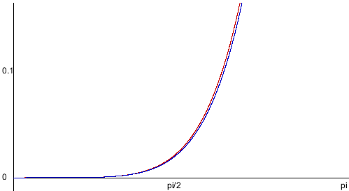
|
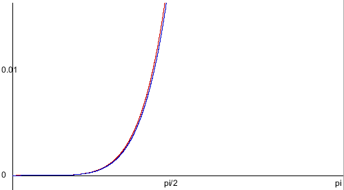
|
| max deflection using unit scale | max deflection at 10x scale | max deflection at 100x scale |
That doesn't actually appear to be all that much better, so let's look at some numbers, to see what the improvement actually is:
| angle | "improved" deflection | "upper bound" deflection | difference |
|---|---|---|---|
| 1/8 π | 6.202833502388927E-8 | 6.657161222278773E-8 | 4.5432771988984655E-9 |
| 1/4 π | 3.978021202111215E-6 | 4.246252911066506E-6 | 2.68231708955291E-7 |
| 3/8 π | 4.547652269037972E-5 | 4.8397483513262785E-5 | 2.9209608228830675E-6 |
| 1/2 π | 2.569196199214696E-4 | 2.7251652752280364E-4 | 1.559690760133403E-5 |
| 5/8 π | 9.877526288810667E-4 | 0.0010444175859711802 | 5.666495709011343E-5 |
| 3/4 π | 0.00298164978679627 | 0.0031455628414580605 | 1.6391305466179062E-4 |
| 7/8 π | 0.0076323182807019885 | 0.008047777909948373 | 4.1545962924638413E-4 |
| π | 0.017362185964043708 | 0.018349016519545902 | 9.86830555502194E-4 |
As we can see, the increase in precision is not particularly big: for a quarter circle (π/2) the traditional k will be off by 2.75 pixels on a circle with radius 10,000 pixels, whereas this "better" fit will be off by 2.56 pixels. And while that's certainly an almost 10% improvement, it's also nowhere near enough of an improvement to make a discernible difference.
At this point it should be clear that while, yes, there are improvement to be had, they're essentially insignificant while also being much more computationally expensive.
TL;DR: just tell me which value I should be using
It depends on what we need to do. If we just want the best value for quarter circles, and we're going to hard code the value for
k, then there is no reason to hard-code the constant k=4/3*tan(pi/8) when you can just as easily hard-code the
constant as k=0.551784777779014 instead.
If you need "the" value for quarter circles, use 0.551785 instead of 0.55228
However, for dynamic arc approximation, in code that tries to fit circular paths using Bézier paths instead, it should be fairly obvious that the simple function involving a tangent computation, two divisions, and one multiplication, is vastly more performant than running all the code we ended writing just to get a 25% lower error value, and most certainly worth preferring over getting the "more accurate" value.
If you need to fit Béziers to circular arcs on the fly, use 4/3 * tan(θ/4)
However, always remember that if you're writing for humans, you can typically use the best of both worlds: as the user interacts with their curves, you should draw their curves instead of drawing approximations of them. If they need to draw circles or circular arcs, draw those, and only approximate them with a Bézier curve when the data needs to be exported to a format that doesn't support those. Ideally with a preview mechanism that highlights where the errors will be, and how large they will be.
If you're writing code for graphics design by humans, use circular arcs for circular arcs
And that's it. We have pretty well exhausted this subject. There are different metrics we could use to find "different best k values", like trying to match arc length (e.g. when we're optimizing for material cost), or minimizing the area between the circular arc and the Bézier curve (e.g. when we're optimizing for inking), or minimizing the rate of change of the Bézier's curvature (e.g. when we're optimizing for curve traversal) and they all yield values that are so similar that it's almost certainly not worth it. (For instance, for quarter circle approximations those values are 0.551777, 0.5533344, and 0.552184 respectively. Much like the 0.551785 we get from minimizing the maximum deflection, none of these values are significantly better enough to prefer them over the upper bound value).
Approximating Bézier curves with circular arcs
Let's look at doing the exact opposite of the previous section: rather than approximating circular arc using Bézier curves, let's approximate Bézier curves using circular arcs.
We already saw in the section on circle approximation that this will never yield a perfect equivalent, but sometimes you need circular arcs, such as when you're working with fabrication machinery, or simple vector languages that understand lines and circles, but not much else.
The approach is fairly simple: pick a starting point on the curve, and pick two points that are further along the curve. Determine the circle that goes through those three points, and see if it fits the part of the curve we're trying to approximate. Decent fit? Try spacing the points further apart. Bad fit? Try spacing the points closer together. Keep doing this until you've found the "good approximation/bad approximation" boundary, record the "good" arc, and then move the starting point up to overlap the end point we previously found. Rinse and repeat until we've covered the entire curve.
We already saw how to fit a circle through three points in the section on creating a curve from three points, and finding the arc through those points is straight-forward: pick one of the three points as start point, pick another as an end point, and the arc has to necessarily go from the start point, to the end point, over the remaining point.
So, how can we convert a Bézier curve into a (sequence of) circular arc(s)?
- Start at
t=0 - Pick two points further down the curve at some value
m = t + nande = t + 2n - Find the arc that these points define
-
Determine how close the found arc is to the curve:
- Pick two additional points
e1 = t + n/2ande2 = t + n + n/2. -
These points, if the arc is a good approximation of the curve interval chosen, should lie
onthe circle, so their distance to the center of the circle should be the same as the distance from any of the three other points to the center. -
For point points, determine the (absolute) error between the radius of the circle, and the
actualdistance from the center of the circle to the point on the curve. - If this error is too high, we consider the arc bad, and try a smaller interval.
- Pick two additional points
The result of this is shown in the next graphic: we start at a guaranteed failure: s=0, e=1. That's the entire curve. The midpoint is
simply at t=0.5, and then we start performing a
binary search.
- We start with
low=0,mid=0.5andhigh=1 -
That'll fail, so we retry with the interval halved:
{0, 0.25, 0.5}- If that arc's good, we move back up by half distance:
{0, 0.375, 0.75}. - However, if the arc was still bad, we move down by half the distance:
{0, 0.125, 0.25}.
- If that arc's good, we move back up by half distance:
- We keep doing this over and over until we have two arcs, in sequence, of which the first arc is good, and the second arc is bad. When we find that pair, we've found the boundary between a good approximation and a bad approximation, and we pick the good arc.
The following graphic shows the result of this approach, with a default error threshold of 0.5, meaning that if an arc is off by a combined half pixel over both verification points, then we treat the arc as bad. This is an extremely simple error policy, but already works really well. Note that the graphic is still interactive, and you can use your up and down arrow keys keys to increase or decrease the error threshold, to see what the effect of a smaller or larger error threshold is.
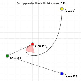
With that in place, all that's left now is to "restart" the procedure by treating the found arc's end point as the new to-be-determined arc's starting point, and using points further down the curve. We keep trying this until the found end point is for t=1, at which point we are done. Again, the following graphic allows for up and down arrow key input to increase or decrease the error threshold, so you can see how picking a different threshold changes the number of arcs that are necessary to reasonably approximate a curve:
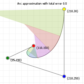
So... what is this good for? Obviously, if you're working with technologies that can't do curves, but can do lines and circles, then the answer is pretty straightforward, but what else? There are some reasons why you might need this technique: using circular arcs means you can determine whether a coordinate lies "on" your curve really easily (simply compute the distance to each circular arc center, and if any of those are close to the arc radii, at an angle between the arc start and end, bingo, this point can be treated as lying "on the curve"). Another benefit is that this approximation is "linear": you can almost trivially travel along the arcs at fixed speed. You can also trivially compute the arc length of the approximated curve (it's a bit like curve flattening). The only thing to bear in mind is that this is a lossy equivalence: things that you compute based on the approximation are guaranteed "off" by some small value, and depending on how much precision you need, arc approximation is either going to be super useful, or completely useless. It's up to you to decide which, based on your application!
B-Splines
No discussion on Bézier curves is complete without also giving mention of that other beast in the curve design space: B-Splines. Easily confused to mean Bézier splines, that's not actually what they are; they are "basis function" splines, which makes a lot of difference, and we'll be looking at those differences in this section. We're not going to dive as deep into B-Splines as we have for Bézier curves (that would be an entire primer on its own) but we'll be looking at how B-Splines work, what kind of maths is involved in computing them, and how to draw them based on a number of parameters that you can pick for individual B-Splines.
First off: B-Splines are piecewise, polynomial interpolation curves, where the "single curve" is built by performing polynomial interpolation over a set of points, using a sliding window of a fixed number of points. For instance, a "cubic" B-Spline defined by twelve points will have its curve built by evaluating the polynomial interpolation of four points, and the curve can be treated as a lot of different sections, each controlled by four points at a time, such that the full curve consists of smoothly connected sections defined by points {1,2,3,4}, {2,3,4,5}, ..., {8,9,10,11}, and finally {9,10,11,12}, for eight sections.
What do they look like? They look like this! Tap on the graphic to add more points, and move points around to see how they map to the spline curve drawn.
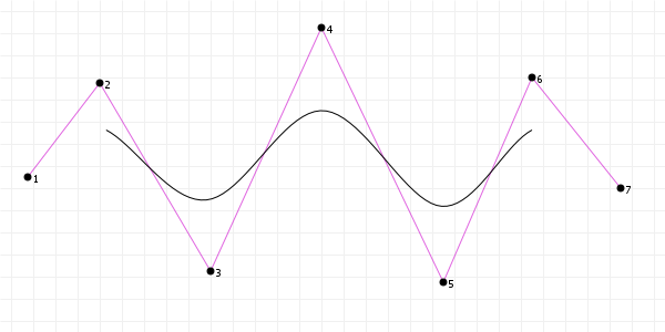
The important part to notice here is that we are not doing the same thing with B-Splines that we do for poly-Béziers or Catmull-Rom curves: both of the latter simply define new sections as literally "new sections based on new points", so a 12 point cubic poly-Bézier curve is actually impossible, because we start with a four point curve, and then add three more points for each section that follows, so we can only have 4, 7, 10, 13, 16, etc. point Poly-Béziers. Similarly, while Catmull-Rom curves can grow by adding single points, this addition of a single point introduces three implicit Bézier points. Cubic B-Splines, on the other hand, are smooth interpolations of each possible curve involving four consecutive points, such that at any point along the curve except for our start and end points, our on-curve coordinate is defined by four control points.
Consider the difference to be this:
- for Bézier curves, the curve is defined as an interpolation of points, but:
- for B-Splines, the curve is defined as an interpolation of curves.
In fact, let's look at that again, but this time with the base curves shown, too. Each consecutive four points define one curve:
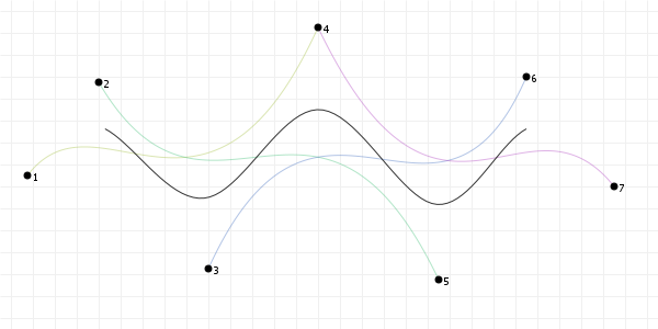
In order to make this interpolation of curves work, the maths is necessarily more complex than the maths for Bézier curves, so let's have a look at how things work.
How to compute a B-Spline curve: some maths
Given a B-Spline of degree d and thus order k=d+1 (so a quadratic B-Spline is degree 2 and order 3, a cubic
B-Spline is degree 3 and order 4, etc) and n control points P0 through Pn-1, we can compute a point on the curve for some value t in the interval [0,1] (where 0 is the start of the curve, and 1 the
end, just like for Bézier curves), by evaluating the following function:

Which, honestly, doesn't tell us all that much. All we can see is that a point on a B-Spline curve is defined as "a mix of all the control
points, weighted somehow", where the weighting is achieved through the N(...) function, subscripted with an obvious parameter
i, which comes from our summation, and some magical parameter k. So we need to know two things: 1. what does
N(t) do, and 2. what is that k? Let's cover both, in reverse order.
The parameter k represents the "knot interval" over which a section of curve is defined. As we learned earlier, a B-Spline
curve is itself an interpolation of curves, and we can treat each transition where a control point starts or stops influencing the total
curvature as a "knot on the curve". Doing so for a degree d B-Spline with n control point gives us
d + n + 1 knots, defining d + n intervals along the curve, and it is these intervals that the above
k subscript to the N() function applies to.
Then the N() function itself. What does it look like?

So this is where we see the interpolation: N(t) for an (i,k) pair (that is, for a step in the above summation, on a specific
knot interval) is a mix between N(t) for (i,k-1) and N(t) for (i+1,k-1), so we see that this is a recursive
iteration where i goes up, and k goes down, so it seem reasonable to expect that this recursion has to stop at
some point; obviously, it does, and specifically it does so for the following i/k values:

And this function finally has a straight up evaluation: if a t value lies within a knot-specific interval once we reach a
k=1 value, it "counts", otherwise it doesn't. We did cheat a little, though, because for all these values we need to scale
our t value first, so that it lies in the interval bounded by knots[d] and knots[n], which are the
start point and end point where curvature is controlled by exactly order control points. For instance, for degree 3 (=order
4) and 7 control points, with knot vector [1,2,3,4,5,6,7,8,9,10,11], we map t from [the interval 0,1] to the interval [4,8],
and then use that value in the functions above, instead.
Can we simplify that?
We can, yes.
People far smarter than us have looked at this work, and two in particular —
Maurice Cox and
Carl de Boor — came to a mathematically pleasing solution: to compute a point
P(t), we can compute this point by evaluating d(t) on a curve section between knots i and i+1:

This is another recursive function, with k values decreasing from the curve order to 1, and the value α (alpha) defined by:

That looks complicated, but it's not. Computing alpha is just a fraction involving known, plain numbers. And, once we have our alpha
value, we also have (1-alpha) because it's a trivial subtraction. Computing the d() function is thus mostly a
matter of computing pretty simple arithmetical statements, with some caching of results so we can refer to them as we recurve. While the
recursion might see computationally expensive, the total algorithm is cheap, as each step only involves very simple maths.
Of course, the recursion does need a stop condition:

So, we actually see two stopping conditions: either i becomes 0, in which case d() is zero, or
k becomes zero, in which case we get the same "either 1 or 0" that we saw in the N() function above.
Thanks to Cox and de Boor, we can compute points on a B-Spline pretty easily using the same kind of linear interpolation we saw in de
Casteljau's algorithm. For instance, if we write out d() for i=3 and k=3, we get the following
recursion diagram:

That is, we compute d(3,3) as a mixture of d(2,3) and d(2,2), where those two are themselves a
mixture of d(1,3) and d(1,2), and d(1,2) and d(1,1), respectively, which are
themselves a mixture of etc. etc. We simply keep expanding our terms until we reach the stop conditions, and then sum everything back up.
It's really quite elegant.
One thing we need to keep in mind is that we're working with a spline that is constrained by its control points, so even though the
d(..., k) values are zero or one at the lowest level, they are really "zero or one, times their respective control point", so
in the next section you'll see the algorithm for running through the computation in a way that starts with a copy of the control point
vector and then works its way up to that single point, rather than first starting "on the left", working our way "to the right" and then
summing back up "to the left". We can just start on the right and work our way left immediately.
Running the computation
Unlike the de Casteljau algorithm, where the t value stays the same at every iteration, for B-Splines that is not the case,
and so we end having to (for each point we evaluate) run a fairly involving bit of recursive computation. The algorithm is discussed on
this Michigan Tech page, but an easier to read version
is implemented by b-spline.js, so we'll look at its code.
Given an input value t, we first map the input to a value from the domain [0,1] to the domain
[knots[degree], knots[knots.length - 1 - degree]. Then, we find the section number s that this mapped
t value lies on:
| 1 | |
| 2 | |
| 3 |
after running this code, s is the index for the section the point will lie on. We then run the algorithm mentioned on the MU
page (updated to use this description's variable names):
| 1 | |
| 2 | |
| 3 | |
| 4 | |
| 5 | |
| 6 | |
| 7 | |
| 8 | |
| 9 | |
| 10 |
(A nice bit of behaviour in this code is that we work the interpolation "backwards", starting at i=s at each level of the
interpolation, and we stop when i = s - order + level, so we always end up with a value for i such that those
v[i-1] don't try to use an array index that doesn't exist)
Open vs. closed paths
Much like poly-Béziers, B-Splines can be either open, running from the first point to the last point, or closed, where the first and last
point are the same coordinate. However, because B-Splines are an interpolation of curves, not just points, we can't simply make the first
and last point the same, we need to link as many points as are necessary to form "a curve" that the spline performs interpolation with. As
such, for an order d B-Spline, we need to make the first and last d points the same. This is of course hardly
more work than before (simply append points.splice(0,d) to points) but it's important to remember that you need
more than just a single point.
Of course if we want to manipulate these kind of curves we need to make sure to mark them as "closed" so that we know the coordinate for
points[0] and points[n-k] etc. don't just happen to have the same x/y values, but really are the same
coordinate, so that manipulating one will equally manipulate the other, but programming generally makes this really easy by storing
references to points, rather than copies (or other linked values such as coordinate weights, discussed in the NURBS section) rather than
separate coordinate objects.
Manipulating the curve through the knot vector
The most important thing to understand when it comes to B-Splines is that they work because of the concept of a knot vector. As mentioned above, knots represent "where individual control points start/stop influencing the curve", but we never looked at the values that go in the knot vector. If you look back at the N() and a() functions, you see that interpolations are based on intervals in the knot vector, rather than the actual values in the knot vector, and we can exploit this to do some pretty interesting things with clever manipulation of the knot vector. Specifically there are four things we can do that are worth looking at:
- we can use a uniform knot vector, with equally spaced intervals,
- we can use a non-uniform knot vector, without enforcing equally spaced intervals,
- we can collapse sequential knots to the same value, locally lowering curve complexity using "null" intervals, and
- we can form a special case non-uniform vector, by combining (1) and (3) to for a vector with collapsed start and end knots, with a uniform vector in between.
Uniform B-Splines
The most straightforward type of B-Spline is the uniform spline. In a uniform spline, the knots are distributed uniformly over the entire curve interval. For instance, if we have a knot vector of length twelve, then a uniform knot vector would be [0,1,2,3,...,9,10,11]. Or [4,5,6,...,13,14,15], which defines the same intervals, or even [0,2,3,...,18,20,22], which also defines the same intervals, just scaled by a constant factor, which becomes normalised during interpolation and so does not contribute to the curvature.
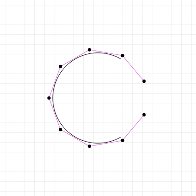
This is an important point: the intervals that the knot vector defines are relative intervals, so it doesn't matter if every interval is size 1, or size 100 - the relative differences between the intervals is what shapes any particular curve.
The problem with uniform knot vectors is that, as we need order control points before we have any curve with which we can
perform interpolation, the curve does not "start" at the first point, nor "ends" at the last point. Instead there are "gaps". We can get
rid of these, by being clever about how we apply the following uniformity-breaking approach instead...
Reducing local curve complexity by collapsing intervals
Collapsing knot intervals, by making two or more consecutive knots have the same value, allows us to reduce the curve complexity in the
sections that are affected by the knots involved. This can have drastic effects: for every interval collapse, the curve order goes down,
and curve continuity goes down, to the point where collapsing order knots creates a situation where all continuity is lost
and the curve "kinks".
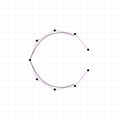
Open-Uniform B-Splines
By combining knot interval collapsing at the start and end of the curve, with uniform knots in between, we can overcome the problem of the curve not starting and ending where we'd kind of like it to:
For any curve of degree D with control points N, we can define a knot vector of length N+D+1 in
which the values 0 ... D+1 are the same, the values D+1 ... N+1 follow the "uniform" pattern, and the values
N+1 ... N+D+1 are the same again. For example, a cubic B-Spline with 7 control points can have a knot vector
[0,0,0,0,1,2,3,4,4,4,4], or it might have the "identical" knot vector [0,0,0,0,2,4,6,8,8,8,8], etc. Again, it is the relative differences
that determine the curve shape.
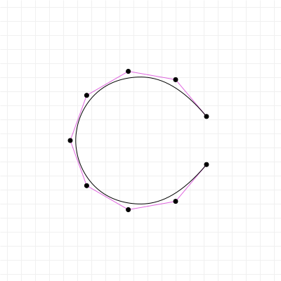
Non-uniform B-Splines
This is essentially the "free form" version of a B-Spline, and also the least interesting to look at, as without any specific reason to
pick specific knot intervals, there is nothing particularly interesting going on. There is one constraint to the knot vector, other than
that any value knots[k+1] should be greater than or equal to knots[k].
One last thing: Rational B-Splines
While it is true that this section on B-Splines is running quite long already, there is one more thing we need to talk about, and that's "Rational" splines, where the rationality applies to the "ratio", or relative weights, of the control points themselves. By introducing a ratio vector with weights to apply to each control point, we greatly increase our influence over the final curve shape: the more weight a control point carries, the closer to that point the spline curve will lie, a bit like turning up the gravity of a control point, just like for rational Bézier curves.
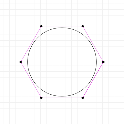
Of course this brings us to the final topic that any text on B-Splines must touch on before calling it a day: the NURBS, or Non-Uniform Rational B-Spline (NURBS is not a plural, the capital S actually just stands for "spline", but a lot of people mistakenly treat it as if it is, so now you know better). NURBS is an important type of curve in computer-facilitated design, used a lot in 3D modelling (typically as NURBS surfaces) as well as in arbitrary-precision 2D design due to the level of control a NURBS curve offers designers.
While a true non-uniform rational B-Spline would be hard to work with, when we talk about NURBS we typically mean the Open-Uniform Rational B-Spline, or OURBS, but that doesn't roll off the tongue nearly as nicely, and so remember that when people talk about NURBS, they typically mean open-uniform, which has the useful property of starting the curve at the first control point, and ending it at the last.
Extending our implementation to cover rational splines
The algorithm for working with Rational B-Splines is virtually identical to the regular algorithm, and the extension to work in the control point weights is fairly simple: we extend each control point from a point in its original number of dimensions (2D, 3D, etc.) to one dimension higher, scaling the original dimensions by the control point's weight, and then assigning that weight as its value for the extended dimension.
For example, a 2D point (x,y) with weight w becomes a 3D point (w * x, w * y, w).
We then run the same algorithm as before, which will automatically perform weight interpolation in addition to regular coordinate interpolation, because all we've done is pretended we have coordinates in a higher dimension. The algorithm doesn't really care about how many dimensions it needs to interpolate.
In order to recover our "real" curve point, we take the final result of the point generation algorithm, and "unweigh" it: we take the
final point's derived weight w' and divide all the regular coordinate dimensions by it, then throw away the weight
information.
Based on our previous example, we take the final 3D point (x', y', w'), which we then turn back into a 2D point by computing
(x'/w', y'/w'). And that's it, we're done!


First off, if you enjoyed this book, or you simply found it useful for something you were trying to get done, and you were wondering how to let me know you appreciated this book, you have two options: you can either head on over to the Patreon page for this book, or if you prefer to make a one-time donation, head on over to the buy Pomax a coffee page. This work has grown from a small primer to a 70-plus print-page-equivalent reader on the subject of Bézier curves over the years, and a lot of coffee went into the making of it. I don't regret a minute I spent on writing it, but I can always do with some more coffee to keep on writing.
With that said, on to the comments!